Is Efficiency Biased?

Introduction

Suppose that a city is considering building neighborhood parks, each of which costs $1 million to build. The residents of a rich neighborhood are willing to pay $2 million for the park, but the residents of a poor neighborhood are willing to pay only $500,000, less than the cost of construction. Suppose as well that the park increases the well-being of the rich and poor by the same amount. Should the city build a park in the rich neighborhood, the poor neighborhood, both, or neither?1

A dominant policymaking ethos of our time—perhaps the dominant one—is the pursuit of economic efficiency.2 The typical efficiency-based economic analysis of law gives a clear answer: build the park in the rich neighborhood but not the poor neighborhood. Doing so is efficient. This goal of economic efficiency is reflected throughout the law, especially in administrative cost-benefit analysis3 and common law adjudication.4 It has reached such a status that one keen observer has called the notion that economic policy should be efficient (apart from explicitly redistributionist tax and transfer programs) the “Brookings Religion”—that is, the standard goal for policy analysts across the country, as exemplified by the work of the famous think tank in Washington, DC.5 The advocates of economic efficiency point to its ability to grow the size of the economic pie, making everyone better off.6 As they say, a rising tide lifts all boats.7 But efficiency’s critics, especially outside of economics, suggest that efficient policy pays insufficient attention to the needs of the poor.8 This view resonates with critiques of neoliberalism and the “Washington consensus” view that governments should adopt efficient, growth-inducing laws.9

This Article works from within economics itself to describe the hidden meaning of efficiency, identifying the particular bias against the poor in many, but not all, efficient policies. It makes three contributions. First, it introduces a new concept, “legal entitlement neutrality,” that classifies efficient legal rules based on their “bias” toward people of different incomes. Second, it characterizes conditions under which an efficient policy distributes more, less, or the same amount of legal entitlements to the rich and the poor. These conditions produce a heuristic rule: money is neutral. Otherwise, efficient policies are probably biased toward the rich. That is, in many cases—discernable based on criteria in this Article—one of the dominant paradigms in the law is biased against the poor, which is a particular concern given rising dissatisfaction with economic inequality as exemplified by the interest in the work of Thomas Piketty.10 Third, it offers implications for policy. In particular, by showing that efficiency is not just indifferent to the poor but is actually often biased against them, this Article offers an important reason to adopt less efficient legal rules that are less biased against the poor.

Understanding these claims requires some precision in understanding what “efficiency” is. When this Article asks, “Is efficiency biased?,” it refers to “Kaldor-Hicks efficiency,” the typical definition used in economic analysis of the law. Kaldor-Hicks (K-H) efficiency maximizes individuals’ willingness to pay for a policy change.11 This goal is particularly associated with scholars like former Judge Richard Posner but is a common goal for setting policies, as it is viewed as maximizing the size of the economic pie. When critics say that efficient policies are biased against the poor, they reference efficiency’s basis in “willingness to pay.”12 Because the rich have greater wealth, the view goes, they will tend to have a greater willingness to pay, and therefore policymakers maximizing efficiency will choose policies that benefit the rich over the poor.

In the 1970s and 1980s, when the efficiency norm rose to dominance in the economic analysis of the law, there was vigorous critique of the alleged bias of efficient policies against the poor.13 But remarkably, this foundational critique of the most common goal in the economic analysis of law, if not in all analysis of law, never quite crystallized. Opponents came up with powerful examples of bias against the poor, and had a strong intuitive account, but never reached a general critique of efficient policymaking’s biased distribution that carefully considered qualifications.14 Rather, the question largely went into hibernation. By revealing the inner workings of K-H efficiency and its application to legal rules, this Article provides that general critique but also qualifies earlier critiques, showing that efficiency is more complex than either its supporters or critics suggest.

The debate about bias in efficient policymaking went into hibernation in part because a view took hold among economic analysts that distributional consequences of efficient policies were inconsequential because taxes and transfers either should or do address distributional concerns.15 The mantra is to have efficient policies that may harm the poor, grow the economic pie as large as possible, and then slice the pie equitably by redistributing to the poor through taxes16 to address distributional concerns.17 That is, if the tax system achieves the appropriate distribution of income, then the distributive impacts of nontax policies do not matter.18

This Article makes a different—and, in the context of economic analysis, uncommon—assumption: the distributional consequences of policies “stick,” as a variety of political frictions described by political scientists suggests could be the case.19 A policy that hurts the poor does not lead to increased transfers to the poor, and a policy that benefits the poor does not lead to increased taxes on the poor. As a result, policies’ distributional impacts matter. What assumption is empirically correct is an open question, but this Article works out the implications under the plausible notion that distributional impacts stick.

In this context, this Article introduces the concept of “legal entitlement neutrality,” which means that, if one’s income changes, one’s efficient allocation of legal entitlements does not change. It thus classifies policies by their tendency to assign a larger or smaller amount of legal entitlements to different individuals on the basis of their income. By “legal entitlement,” this Article means stuff that the government allocates—for example, clean air, provision of parks, spending on infrastructure, or road safety. Legal entitlement neutrality is primarily a question of “fairness” in allocation: For a given type of efficient policy, do richer people tend to get more, less, or the same amount of stuff?

Two things should be noted about legal entitlement neutrality. First, “neutrality” in this Article refers specifically to this concept, not some broader platonic concept of neutrality. For example, in the view of many, a policy that increases well-being equally for everyone would probably need to give more money to the poor than to the rich because a dollar may buy more well-being for the poor than for the rich, owing to the rich’s greater resources.20 Bias here refers to an allocation of goods and services, not utility. Second, it refers only to efficient policies, not to other types of policies, which are not characterized by a presence or lack of legal entitlement neutrality.

Efficient policies can be “poor-biased,” “rich-biased,” or “neutral.” A policy is poor-biased if, as one gets richer, one gets fewer legal entitlements from efficient legal policies. For these policies, the poor are willing to pay more than the rich for the legal entitlements (such as public bus routes, perhaps), so efficient legal rules endow the poor with more of them. Poor-biased policies are rare because it is unusual for the poor to be willing to pay more for anything than the rich. As a result, this Article focuses on the division between the more frequent rich-biased and neutral policies.

An efficient policy is rich-biased if, as one gets richer, one tends to get more legal entitlements from efficient policies.21 For these policies, the rich have a greater willingness to pay for the legal entitlement than the poor, so efficient policies endow the rich with more of them. There are lots of rich-biased policies because there are lots of things that the rich are willing to pay more for than the poor.22

An efficient policy is neutral if, as one gets richer, efficient legal rules do not change one’s legal entitlements. In particular, everyone has the same willingness to pay for one dollar in increased or decreased income: everyone’s willingness to pay for $1 is $1. Neutral policies are common in the law. For example, the willingness to pay of two identical laundromats, one owned by a rich person and the other by a poor person, to stop pollution from a neighboring factory that is reducing the laundromats’ profits by $1 does not depend upon the laundromat owners’ incomes. Both owners are willing to pay $1 to avoid the harm. Generally, business contexts that shift profits from one business to another (for example, in tort, contract, and corporate law) are neutral because everyone has the same willingness to pay for a dollar of profit. As this Article argues, subtle differences in policy context can lead to big differences in bias.

While any given neutral policy may benefit the rich or the poor, neutral policies grow the size of the economic pie without systematic bias toward the rich or the poor. It is thus plausible to believe that they have distributional impacts that even out across many policies. Such a belief is not reasonable for rich-biased policies, which systematically, as a matter of methodology, distribute more to the rich. After revealing this hidden division, this Article illustrates it using an extended example involving tort liability. The underlying math is described in the Appendix.

Notwithstanding this division between policies, overall efficiency analysis places a heavy thumb on the scale in favor of rich-biased policies because the rich—due to their greater wealth—are generally willing to pay more for the things that legal entitlements confer.23 Thus, rather than allocating resources to the poor, who are most in need, efficient policies tend to do the opposite: allocating resources to the rich, who are willing to pay the most. Efficient policies will therefore tend to allocate more valuable legal entitlements to the rich: more spending on transportation, more parks, and cleaner air in rich places than in poor ones. This Article calls this phenomenon the “rich get richer” principle of law and economics. In effect, unless their distributional consequences are offset, efficient polices tend to reinforce the existing wealth distribution: greater ownership of wealth entitles individuals to a larger allocation of policy entitlements—even if the rich do not pay for it.24 That is, rich-biased policies give disproportionate legal entitlements to the rich for free, exacerbating inequality.

Legal entitlement neutrality is important because many believe that at least some areas of government policymaking should not give more or fewer legal entitlements to people on the basis of their income. In particular, many hold the view that certain branches of government (often the courts and administrative agencies) should not redistribute,25 redistribution being the exclusive province of the legislature. Efficient policies, which often redistribute toward the rich, may seem problematic not only to those who favor redistribution to the poor but also to others, such as libertarians, who do not want the government to treat people differently because of their income, or to those who are concerned about the legitimacy of the state.26

A detailed discussion of policy implications is beyond the scope of this Article. But the analysis does suggest a two-point rubric for addressing the distributional impacts of efficient policies. This Article provides guidance on when and why to consider adopting inefficient policies if one wishes to both avoid redistributing toward the rich and adopt policies that make everyone better off. The rubric can be applied whenever the law considers efficiency.

The first and threshold question is whether the context is one that is likely to lead to a rich-biased rule. For neutral policies, distributional impacts may even out over time: as a matter of methodology, there is no bias. For rich-biased policies, however, there is an inherent legal entitlement bias. Second, does the institutional context suggest that policies’ distributional effects will be offset or be sticky? For example, legislatures can more easily adjust policies to address distributional concerns; administrative agencies and courts are less able to do so, making it more likely that the perverse distributional consequences described here will stick.27 If the efficient policy is rich-biased and has distributional impacts that are sticky—and if we hold one of the broad range of normative commitments suggesting that distributing more legal entitlements to the rich without the rich paying for them is perverse—then such a policy should not be adopted. Instead, policy alternatives that are explicitly inefficient, with a goal of putting the rich and the poor on equal footing, should be adopted.

This Article proceeds as follows. Part I describes the precise meaning of efficiency. Part II describes the traditional view that policies should maximize efficiency, with distributional impacts addressed by taxes and transfers. This Article then departs from that conventional view by supposing that policies’ distributional impacts stick, making the distributive impacts of efficient policies an essential question. Part III introduces “legal entitlement neutrality” and illustrates the concept with examples. Part IV offers real-world illustrations of rich-biased policies from administrative law and torts. Part V discusses potential policy responses. Part VI responds to potential critiques.

I. Efficiency: An Explanation

Kaldor-Hicks efficiency is the typical metric used in law and economics and is the primary subject of this Article. Throughout this Article, references to “efficiency” or “efficiency analysis” mean K-H efficiency unless otherwise noted. K-H efficiency (also sometimes called “cost-benefit analysis”28 ) measures the willingness to pay of the parties affected by various policy options and then chooses the policy that maximizes the sum of the willingness to pay of those parties. (This Part gives an intuitive explanation, leaving the technical, mathematical definition of K-H efficiency to the Appendix.) By choosing policies most responsive to people’s preferences (as reflected by their willingness to pay), K-H efficiency thus maximizes preference satisfaction given both the current distribution of income and the constraints, like a limited budget, under which policymakers operate.29 Doing so maximizes so-called “social surplus,” or just “surplus”: people’s total willingness to pay for a given social arrangement.30

The desirability of K-H efficiency is based in part on the notion that it is relatively observable. In particular, unlike utility or well-being, which are not directly observable, willingness to pay is, at least in principle. The reason is that, in real-world markets, we observe people paying for things, and if someone pays for something, presumably she is willing to pay for it. Thus, by allocating legal entitlements to people who are willing to pay for them, K-H efficiency seeks the arrangement of goods, services, and externalities that the free market would achieve, taking the current wealth distribution as given.31 However, unlike in markets, in which parties actually pay for what they receive, K-H efficiency asks about hypothetical willingness to pay. That is, K-H efficiency is not about what parties did pay, but rather what they would have paid, and it does not require that people actually pay for what they receive.

Put a different way, by seeking to maximize willingness to pay,32 efficiency analysis promotes the allocation of goods, services, and externalities that would result if there were free bargaining and everyone who gained from the new policy compensated those who lost, whether or not the compensation actually takes place. If two parties are affected by a policy change, and one party would be willing to pay more for a policy change than another party would be willing to pay to avoid the change, the policy is efficient—regardless of whether there is actually a transfer from the beneficiary to the harmed party.33 Adopting an efficient policy ensures the total amount that people are willing to pay in aggregate for policies has increased. As former Judge Posner famously put it, in a sense, “wealth” has increased34 —not in that people have more money in their bank accounts, but rather in the sense of total surplus (willingness to pay for social arrangements) increasing. Adopting such efficient policies then respects people’s preferences by adopting the policies that they value most.

K-H efficiency is different from two other concepts also used for economic analysis. The first is Pareto efficiency.35 A policy is Pareto efficient if there is no alternative policy that makes someone better off without making anyone worse off.36 A policy that is Pareto efficient is thus an improvement on the status quo. However, Pareto efficiency has been criticized as unhelpful because, for most policies, making no one worse off is impossible due to the large number of people involved.37 Part of the appeal of K-H efficiency is that it delivers policy recommendations without the very stringent requirement that no one be made worse off. Indeed, K-H efficiency is also sometimes called “potential Pareto efficiency” because it is viewed as identifying changes that increase overall surplus and thus have the “potential” to be Pareto efficient after transfers from those who gain from the policy change to those who lose from it.38

Another concept used in economic analysis is “social welfare” or well-being. Though the goal can take a variety of forms, most typical is developing a measure of each individual’s utility level, summing those, and then choosing the policy that maximizes that sum of utilities (which potentially can be weighted).39 There are a variety of ways that social welfare maximization can differ from efficiency analysis. For this Article’s purposes, the most important way is that allocating money, goods, or other forms of legal entitlements to individuals with low incomes may increase utility because of the declining marginal utility of income resulting from money being less valuable to rich people, a conventional assumption in economics.40 Efficiency analysis, in contrast, does not directly consider the declining marginal utility of income and thus does not systematically allocate resources to the poor.

Some—most famously, Posner in the 1970s and 1980s—take K-H efficiency as the ultimate goal of government policy.41 More commonly, though, law and economics scholars take well-being as the ultimate goal of policy but nevertheless support efficient policymaking in many arenas for at least one of two reasons. The first is that efficiency maximizes the size of the economic pie that taxes and transfers can then redistribute to address concerns about distribution. Part II discusses that argument. Another argument is that, across a large number of efficient policies, distributional consequences will even out.42 The rich will benefit from some policies and the poor from others. But across a large enough number of policies, everyone is better off. So the best way to maximize welfare is to adopt efficient policies, which will ultimately maximize welfare. This view should be familiar to anyone who even occasionally reads the news and is associated with comments like “a rising tide lifts all boats”43 and (among critics) “trickle-down economics.”44

This popular view in support of efficiency has an analogous popular view opposed to it, often associated with critics of neoliberalism, who argue that efficiency pays insufficient attention to the needs of the poor.45 Perhaps most famously to legal scholars, Ronald Dworkin gave the examples of Derek and Amartya.46 Derek is poor, and Amartya is rich. Derek has a book that Amartya would like. Because of his poverty, Derek would be willing to part with the book, which he holds dearly, for $2. Amartya, though he is not very interested in the book, is willing to pay $3 for the book due to his great wealth. Thus, Dworkin points out that it would be efficiency-maximizing for the government to take the book from poor Derek and give it to rich Amartya, even without compensation.47 Rich Amartya is getting something from the government just because he’s rich, not because his well-being is enhanced more by having it.

This analysis is helpful so far as it goes—especially for making Dworkin’s point that utility and efficiency are quite different things. But it—along with other analyses from economists48 —leaves many questions unanswered, as it is just one example that does not extend to the huge range of issues to which efficiency analysis is applied. How broad is the critique? Are there exceptions? Is this just a narrow case?49 Tracing out more precisely the distributive implications of efficient policymaking is the task of this Article.

II. The Distributional Consequences of Policies: A Sticky Take

Law and economics typically justifies the goal of maximizing efficiency by arguing that efficiency actually promotes social welfare maximization because efficient policies maximize the size of the pie that can then be redistributed through taxes. The leading law and economics textbooks make an argument along these lines.50 Thus, there has been little reason for systematic study of distributional impacts of efficient policies, even as efficiency has become the goal of much policymaking and analysis; those distributional impacts have been taken not to matter because they are offset by other policies. This Part explains this conventional reasoning and then turns to the alternative “sticky distribution” assumption introduced in this Article.51

The idea that all policies except tax policy should ignore distributional effects is long-standing and has an impressive list of proponents, including Nobel Laureate Paul Samuelson,52 foundational scholar of modern public finance Richard A. Musgrave,53 and leading law and economics scholars Louis Kaplow and Steven Shavell.54 The classic argument for this idea in law and economics comes from Kaplow and Shavell. They introduced the “double distortion” argument that adopting an inefficient legal rule to benefit the poor by giving the poor larger damages in torts results in two distortions: both to the behavior being regulated (roads that are “too safe” because of damages that are larger than efficient) and to income earning (people have an incentive to earn less so that they can get larger damages).55 In an argument that has generated disagreement56 but is not the subject of this Article, they say that it is typically welfare-enhancing to adopt the efficient rule and then redistribute through taxes.57 The taxes distort, but they result in only one distortion instead of two, thereby enhancing welfare.

To lay observers, a more familiar example of this argument comes from trade policy. The longtime refrain from economists of (nearly) all stripes has been that countries should adopt free trade, notwithstanding potentially negative impacts on the poor, because trade increases the size of the economic pie, and those gains can be redistributed to the poor through taxes and transfers.58 Both the Kaplow-Shavell torts example and the trade example are driven by the same two-step reasoning: everyone can be made better off through efficient nontax policies plus taxes and transfers.

An assumption about politics that is typically implicit underlies this analysis: those taxes and transfers actually happen so that the political system will recover a fair distribution of income. This Article calls this the “distributional offset” assumption. As Kaplow notes: “There may exist a sort of political equilibrium regarding the extent of redistribution. Thus, there may be a tendency for policies—perhaps not individually, but taken as a whole over a period of time—to be implemented in a distribution-neutral fashion.”59 In other words, normal democratic processes like voting will yield offsetting distributional consequences because voters have preferences for a certain distribution of income and will thus seek to have any distributional consequences of policy changes offset.60

To be clear, few explicitly assert that the distributional offset assumption actually is true. The more common explicit claim in canonical texts is that taxes should be used, rather than that they are used—a normative claim rather than a positive one.61 But law and economics analysis that recommends efficient policies de facto makes that assumption implicitly; if the distributional offset assumption does not hold, then the logic that the distributional consequences do not matter breaks down. For example, an efficient policy may hurt the poor but benefit the rich by more than it hurts the poor. To those who want to promote social welfare, or other social goals, this policy may not be desirable if the distributional offset assumption does not hold.

And indeed, other traditions, in political science and elsewhere, suggest the reasonableness of a “sticky distribution” assumption—that is, that distributional consequences are not offset.62 A full description of this scholarship is beyond the scope of this Article, but it is worth sketching some reasons for why policy may not offset distributional consequences to reproduce an optimal distribution of income in the aftermath of a new policy. One reason is that inertia could arise from a variety of sources, including the many veto points that could thwart democratic will.63 Inertia is aided by the population’s ignorance (possibly rational ignorance64 ) of the specifics of how policies change.65 As a result, an agency or court could make law with distributional consequences that long endure. The distributional consequences over the short and medium run matter in addition to those over the long run; for example, with an 8 percent discount rate, a ten-year delay in offset is closer to no offset than immediate offset.66

Furthermore, the public choice approach raises the question of whether that long run point will ever arrive. Public choice models how economic interests organize themselves to exert influence over policy outcomes through lobbying, donations, and other mechanisms.67 For example, Professor Mancur Olson describes how, given the costs of collective action, small groups with concentrated interests tend to prevail over larger groups with more diffuse interests.68 Groups that receive benefits through policies, efficient or otherwise, may constitute just such entrenched interests, and it may be difficult to use taxes and transfers to benefit more diffuse losers from a policy change. Indeed, to the extent that higher-income groups receive benefits, there is evidence (admittedly contested69 ) suggesting that the preferences of lower-income groups matter little for policymaking and that instead only the preferences of higher-income groups matter.70

Empirically, little is known about whether the distributional impacts of various institutions’ policy choices stick. One piece of evidence shows that, after state courts order increases in school funding that largely benefit the poor, the distributional consequences are not offset at all through taxes or spending, even decades afterwards.71 This evidence is consistent with the sticky distribution assumption but not the distributional offset assumption. Other evidence on the response to court orders on prison spending points the other way: those court orders appear to be funded by cuts to programs benefitting low-income individuals.72

We don’t know the answer to what the best assumption about politics is, and this Article does not take a stand either way. But there is at minimum a plausible case that distributional consequences will not be fully offset. In any case, the correct assumption probably varies depending on institutional context, a point that this Article returns to in Part V. For now, instead of assuming that the distributional impacts of policies are completely offset elsewhere, this Article adopts the sticky distribution assumption. The stakes for this Article are that, unlike under the conventional assumption, the distributional impacts of efficient policies matter.

III. Legal Entitlement Neutrality

With that assumption about politics, this Article asks: What are the distributional consequences of efficient policies? In particular, this Article asks whether efficient policies satisfy the novel but intuitive concept of legal entitlement neutrality. This Article defines “legal entitlement neutrality” as follows: as one’s income increases, efficiency-maximizing policies are no more or less likely to systematically endow one with legal entitlements (including goods, services, or money). (See the Appendix Section B for a mathematical definition.) In other words, legal entitlement neutrality is a question of how stuff is allocated. For example, if you get richer (but stay the same otherwise), do efficient legal rules give you more of an entitlement to clean air? Some may find neutrality an important minimum threshold that courts and agencies should satisfy because, if the distributional consequences of policies stick, then systematically regressive policies would exacerbate inequality. In other words, some may believe that judges and administrative rulemakers ought not be concerned with redistribution and should be neutral with respect to the rich and the poor. This Part shows that the answer to this question about whether policies satisfy legal entitlement neutrality turns crucially on the type of policy under consideration.

Legal entitlement neutrality naturally divides policies into three types. Neutral efficient policies do not change their distribution of legal entitlements to individuals as their income increases. Rich-biased efficient policies distribute more of a legal entitlement to individuals as their income increases. Poor-biased efficient policies distribute less of a legal entitlement to individuals as their income increases. (The Appendix defines these terms mathematically.) As this Part explains, efficiency analysis places a heavy thumb on the scales in favor of rich-biased policies. This Part offers examples of each type of policy in turn and then returns to the generalization of legal entitlement neutrality. The Appendix provides a simple (and novel) formula for understanding what utility functions yield which type of policy and includes graphical representations to help understand the intuition behind this formula.

Before moving on, four clarifications are in order. First, legal entitlement neutrality is a feature of efficient policies; policies that are not efficient are not part of the categorization. Second, legal entitlement neutrality is not a question of whether, in any individual case, an efficient policy benefits richer people or poorer people. For example, as this Article shows, there may be a tort in which a poor person wins, but the legal rule is still neutral. Rather, the question is one of systematic bias as a matter of the methodology of efficiency. Third, legal entitlement neutrality is primarily a question of fairness, not utility. Utility can of course be implicated when people of different income groups receive different legal entitlements—and this Part discusses those implications. But one need not think in utility terms to appreciate the insight. Fourth, categorization is an empirical question and is one that uses tools already common (though imperfect) in cost-benefit analysis. Through the various methods that currently are used—such as surveying affected parties or using their market behavior as proxies73 —analysts can measure how willingness to pay changes with income.74 The answer to that question determines categorization: for rich-biased rules, willingness to pay increases as income increases; for neutral rules, willingness to pay stays the same; and for poor-biased rules, willingness to pay decreases at higher incomes.

The following Sections focus on two examples of the tort of nuisance––one neutral and one rich-biased. Both examples apply the “Hand formula”75 in determining whether a polluting factory has failed to meet its duty of care and is thus negligent, requiring it to pay damages; essentially, the costs and benefits of the harm are compared. A polluter pays the cost of its harm if and only if its pollution is inefficient—in other words, if the costs exceed the benefits of the pollution. (A similar analysis could be conducted with federal rulemaking, in deciding whether a rule should be imposed.) A plaintiff receiving damages is equivalent to receiving a legal entitlement—the legal right not to have happen to her whatever the defendant was doing.76 This Article compares the efficient legal treatment of poor and rich people being polluted on, first in a neutral context, with the factory polluting on a laundromat, and then in a rich-biased context, with the factory polluting on homeowners.

A goal of this Article is to show that, while the two examples may seem similar, they are actually examples of different categories of legal rules with very different implications for distribution and potentially very different policy implications. Although the focus is on the contrast between neutral and rich-biased rules, this Article then briefly discusses poor-biased policies, which are uncommon. This Part then turns to the predominance of rich bias in efficient policymaking, which this Article calls the “rich get richer” principle. Finally, this Part shows how to understand these results within a utility framework.

A. Neutral Policies

Consider first the neutral case in which the income of the owner of a laundromat—the party being polluted—does not matter for the efficient legal rule. Like the owner of the factory, the owner of the laundromat is profit-maximizing. To stop the emission of pollution, the factory can install pollution scrubbers at a cost of $5,000 in reduced profits. Thus, the factory’s willingness to pay for the benefit of emitting the pollution is the $5,000 that the factory saves by not putting in the scrubbers.

Of the two possible laundromat owners, start with the rich one. With the pollution, she needs to purchase an air purifier for $10,000 to produce acceptably clean clothes.77 As a result, the laundromat’s willingness to pay to avoid the cost of the pollution is $10,000 in reduced profits. The Hand formula’s efficiency analysis compares the costs and benefits of the pollution, asking: Is it efficient for the polluter to put in the scrubbers? If yes, then the factory is found to have failed to meet its duty of care; it is then held negligent and must pay damages.

Because pollution’s cost ($10,000) exceeds its benefits ($5,000), the efficient legal rule is to impose liability on the factory, holding it negligent in the amount of $10,000. As a result, the factory faces $10,000 in damages from not installing the scrubbers, but needs to pay only $5,000 to install them, so the negligence rule thereby incentivizes the factory to install the scrubbers in the shadow of this prospective rule. Thus, the laundromat de facto has the right to clean air in this case. Column (1) of Table 1 summarizes these facts, with the willingness to pay (WTP) of each party and the resulting efficient legal rule.

Compare that case of a rich owner of the laundromat with the case in which every fact is the same, except that the owner of the identical laundromat is poor. The factory owner still has a cost of $5,000 for installing the scrubbers, so its willingness to pay for the pollution is $5,000. And the cost of the pollution to the laundromat owner is still the need to install an air purifier, which costs $10,000, so her willingness to pay to avoid the pollution is $10,000. The WTP numbers for both parties are the same: the costs of the pollution ($10,000 for the air purifier) exceed the benefits of the pollution ($5,000 for the scrubbers). As a result, the outcome is the same: the factory is negligent. It needs to pay damages, and the laundromat owner has the right to the clean air, as summarized in Column (2) of Table 1.

What drives the analysis is that the laundromat owner’s willingness to pay does not change with her income. A poor owner has the same willingness to pay to avoid pollution as a rich owner does: the cost of installing the air purifier. Thus, regardless of her income, the laundromat owner’s willingness to pay to avoid the pollution is still $10,000.78 As a result, the same analysis applies even though the owner is poor. In this context, the negligence rule is a neutral rule.

Table 1:  Neutral Legal Rule Outcome

Plaintiff income	(1) Rich	(2) Poor
Plaintiff WTP to avoid pollution	$10,000	$10,000
Factory WTP to pollute	$5,000	$5,000
Receives legal entitlement (has higher WTP)	Plaintiff (laundromat)	Plaintiff (laundromat)
Outcome	Factory faces damages and installs scrubbers	Factory faces damages and installs scrubbers

More basically, rich and poor people have the same willingness to pay for a dollar of profit: one dollar. Indeed, it is generally the case that contexts in which dollars are all that matter—most prominently, when profits are all that matter to the parties involved—lead to neutral legal rules. Such rules are present, for example, in the contract or corporate law that governs relations between two businesses, financial regulation, or the panoply of other areas in which only money itself matters. In this example, the income of the owners of the laundromat doesn’t matter for their legal entitlement to clean air. They have the same willingness to pay to avoid the cost of the air purifier: $10,000 because $10,000 is worth $10,000 to both a rich and a poor person. As a result, the legal rule treats rich and poor people the same.

Finally, consider two aspects of the economic pie, the size of which neutral efficient legal rules are maximizing. First, this economic pie consists of money. When the efficient legal rule is adopted, the economy produces more dollars. In this example, with the efficient legal rule, instead of forcing the laundromat to spend $10,000 on an air purifier, the factory installs the scrubbers for $5,000, producing an extra $5,000 of money. Second, any given policy may benefit the rich or benefit the poor. For example, poor people benefit from the rule if the laundromat owners are poor, and rich people benefit if the laundromat owners are rich. But across a large number of efficient policies, the distributional impacts of such neutral legal rules could plausibly even out. Because any individual efficient legal rule has no bias, in aggregate many such rules may not have systematic distributional impacts.

B. Rich-Biased Policies

Contrast this neutral context with a rich-biased context. Suppose that the same factory is involved with the same pollution and the same potential air scrubbers. But suppose that, instead of polluting a laundromat, the factory is polluting homeowners whose health is harmed by the smog caused by the pollution.79 (To make the example as stark as possible, assume that the pollution makes people feel ill but does not harm their productivity as workers.) Consider the efficient liability rule here.80 Once again, start with a rich person. Rich people tend to be willing to pay a relatively large amount for amenities like clean air that produce good health.81 Suppose that a rich person is willing to pay $10,000 for clean air. Because the costs and benefits are the same as the two cases (rich and poor) involving the laundromat, the same efficient legal rule results. The $10,000 in costs from the pollution exceeds the $5,000 in benefits from the pollution, so liability is imposed on the polluter. In the shadow of this liability, the factory will install the scrubbers, and the homeowner will have the right to clean air. See Column (1) in Table 2 describing this scenario.

Table 2:  Rich-Biased Legal Rule Outcome

Plaintiff income	(1) Rich	(2) Poor
Plaintiff WTP to avoid pollution	$10,000	$2,500
Factory WTP to pollute	$5,000	$5,000
Receives legal entitlement (has higher WTP)	Plaintiff (homeowner)	Defendant (factory)
Outcome	Factory faces damages and installs scrubbers	Homeowner polluted on without compensation

Contrast a rich homeowner with a poor homeowner, again with everything the same except for the income of the homeowner. Poor homeowners tend to be willing to pay less for amenities like clean air. Poor homeowners have limited funds; they have little that they are willing to spend on clean air because they have more pressing things to spend money on—things that the rich themselves have already purchased. Suppose, for example, that the poor homeowner would be willing to pay $2,500 for the clean air. Then the efficient legal rule reverses: it is not efficient to impose liability on the factory because the $2,500 cost of the pollution is less than the $5,000 benefit of the factory not installing the air scrubbers. As a result, the poor homeowner is polluted on without compensation. See Column (2) in Table 2 describing this scenario.

In other words, the rich homeowner but not the poor homeowner has the right to clean air—even though the rich homeowner pays nothing for the right. The liability rule in this context is rich-biased because it is systematically more likely to allocate clean air to the rich than to the poor. This is because the rich are more likely to have a willingness to pay for clean air in excess of the $5,000 cost of installing scrubbers. Homeowners do not pay for the policy, but rich homeowners get the clean air, and poor ones do not. Neutral rules, on the other hand, exhibit no such bias; some may benefit poorer people (for example, when the laundromat owner was poor), and some may benefit richer people (for example, when the laundromat owner was rich), but there’s not a systematic bias across legal rules because income does not matter for legal entitlement allocation.

Consider again the economic pie, the size of which the rich-biased policy is maximizing. For rich-biased policies, unlike neutral policies, money does not constitute the economic pie. We know this because, for the cases of both the rich and poor homeowners, the cost of the scrubbers for the factory—the only money involved in the example because the valuation of good health does not affect anything financial—is the same: $5,000. Yet the efficient outcomes are different: the rich get the clean air, and the poor do not.

It is also not utility that is in the economic pie. It is plausible to think that the rich and the poor have the same utility from clean air. On that assumption, if it is utility-maximizing for the rich to have clean air, then it is also utility-maximizing for the poor to have clean air. (Part III.F illustrates this argument with an example.) Yet the poor do not get clean air in the example, meaning that this efficient arrangement is not necessarily utility-maximizing.

Rather, the economic pie for rich-biased efficient polices, as for all efficient policies, is made up of fictitious willingness to pay units. Let’s call them “WTPs.” For rich-biased policies, basing policy on maximizing the sum of WTPs disadvantages the poor, because the poor can generally afford to pay less for things. Effectively, the preferences of the poor count less than the preferences of the rich for making the WTP pie bigger because the rich are willing to pay more. That disparity is why, even if the rich and the poor have the same dislike of air pollution, when maximizing the size of the economic pie, the rich receive a legal entitlement to clean air while the poor do not.

This bias would matter little if rich-biased policies were rare. But policies that would be rich-biased if they are efficient are ubiquitous among the things that governments provide because the rich tend to be willing to pay more than the poor for goods. Indeed, as Appendix Section D shows, rich-biased goods are equivalent to what economists call “normal” goods, in which demand increases with income. Here are some examples:

• Siting polluting facilities: The main examples in this Section concern tort law and the decision of polluters to install pollution control equipment. State and local governments also have direct approval authority over siting polluting facilities, with similar consequences for pollution in rich versus poor areas: siting more factories in poor areas than in rich ones would be efficient because the poor (in many cases) have a lower willingness to pay to avoid pollution.82
• Public spending on pharmaceutical research: Rich people’s greater willingness to pay for their health makes it efficient to fund more research on diseases that afflict the rich than those that afflict the poor—both within countries and, even more starkly, between countries.83
• Road safety: The rich are likely willing to pay more for safe roads, suggesting efficient torts and spending policies that impose greater penalties when the well-off are harmed and greater public spending in rich areas to avoid such outcomes.84
• Spending on law enforcement and voting: Local governments choosing which neighborhoods receive more money for law enforcement or infrastructure (for example, personnel or machines) to make voting quicker face an inherent bias: rich people are willing to spend more for a marginal decrease in crime or to spend less time voting.85
• Infrastructure like parks or transportation: Legislatures decide whether to build public infrastructure and may choose to do so in richer neighborhoods that have a higher willingness to pay. Take the example of parks in a rich versus a poor neighborhood. The efficient policy is likely to build more parks in rich neighborhoods than in poor ones.86 And legislatures also decide between funding bus mass transit (often used by lower-income individuals, who have a lower willingness to pay) and airports (used on average by higher-income individuals):87 efficient policies will systematically spend more on what rich people want than what poor people want even if a given amount of spending would increase well-being for the rich and the poor by the same amount.

This list could go on. Anecdotally, there is some evidence that, in at least some of these cases, in practice the rich do benefit relative to the poor, who may, for example, be subject to more pollution (at least globally),88 less public pharmaceutical research spending that benefits them,89 more dangerous roads,90 less spending on law enforcement,91 longer waits to vote,92 worse parks,93 and worse transportation infrastructure.94 The point here is not that there actually are disproportionate legal entitlements going to the rich and the poor—much less that efficiency analysis has anything to do with that allocation. Indeed, if more polluting facilities are sited in low-income minority neighborhoods, that could be because of market forces like lower costs of acquiring land, the lack of political power of low-income minority communities, racism, a focus on efficiency-minded thinking, or other factors. It is often impossible to know. The point is that efficiency would justify such allocations—and that such differences in allocation would be large. For example, a recent analysis conducted for the Environmental Protection Agency suggests willingness to pay to avoid mortality roughly doubles as income doubles.95 Thus, it would be efficient to spend about twice as much to save the life of someone earning $120,000 as someone earning $60,000.

C. Poor-Biased Policies

It is not the case that willingness to pay always increases or stays even with income. Rather, some things become more valuable (in WTP terms) as income goes down, and thus poorer people get a larger legal entitlement than rich people under the efficient policy. As Appendix Section D shows, poor-biased goods are equivalent to what economists term “inferior” goods, for which demand increases as income decreases.96 For poor-biased polices, efficiency analysis is also biased but toward poor individuals. An example of a poor-biased policy could be spending on bus-based public transit. Consider a state transportation authority deciding whether to spend more money on buses in a poor city or a rich city of equal populations, each of which currently receives the same amount of state spending on buses. The transportation authority conducts its analysis to determine which city is willing to pay more for the increased spending. It may be that the poor city actually has the greater willingness to pay for the spending on buses because rich people—though they are willing to pay more for most things—are not willing to pay more for buses for the simple reason that they wouldn’t use the buses. They already own their own cars and prefer to use those, while poor people often do not own cars and thus would greatly value the increased availability of buses.97

Poor-biased policies are rare for an intuitive reason: rich people have more money to spend! And for those things on which the rich spend more money, they must be willing to pay more than the poor—or else the rich would not in fact be spending more than the poor. Empirical research on willingness to pay backs up this intuitive explanation.98 Indeed, it is difficult to think of many other plausible examples of poor-biased policies. Another example might be efficient spending by a legislature on building public swimming pools across communities. Spending more in lower-income communities might be efficient if the wealthy would be reluctant to use the pools, perhaps because the well-off can opt to build their own pools at their homes or in their subdivisions.

Even with these examples, the poor-biased policies are subcategories of larger categories of rich-biased policies. Buses are a subcategory of transportation infrastructure, and pools are a subcategory of public amenities infrastructure. That is not a coincidence. In any broad category of efficiency-oriented policy, like transportation infrastructure or public amenities, the rich are likely willing to pay more by virtue of their greater income. For example, the rich may not use buses, but they use roads, bridges, and airports—and are willing to pay quite a lot to commute to and from their well-paying jobs and to travel on vacations. The poor may be willing to spend more on buses but not on infrastructure overall. This result makes sense: the rich have more money to spend. Across all categories of goods, they must be willing to pay more—or else the rich would spend less than the poor. But the narrower the subcategory of overall consumption, the more likely that there will be something that the poor are actually willing to spend more on. When aggregated, however, there likely are few categories for which that is true.

D. Summary

Table 3 summarizes the examples of neutral, rich-biased, and poor-biased rules. The first column has the neutral case, in which the legal entitlement is clean air. The laundromat plaintiff cares about the clean air because the clean air affects the laundromat’s profits. Because everyone values a dollar of profits at a dollar, wealthier laundromat owners have the same willingness to pay for the clean air as the poorer laundromat owners. As a result, the rich do not get more of a legal entitlement. These policies are fairly common—whenever legal rules are determined by profits.

Table 3:  Summary of Neutral, Rich-Biased, and Poor-Biased Rules

	Neutral	Rich-Biased	Poor-Biased
Legal entitlement	Clean air	Clean air	Bus Service
Why care	Profits	Health	Transportation
↑ income -> WTP?	Same	↑	↓
Rich get more legal entitlement?	No	Yes	Poor get more
Frequency	Common	Very common	Uncommon

The second column has the rich-biased legal rule example of homeowners being polluted on by the same factory. It involves the same legal entitlement, clean air, as the neutral rule. But the reason that the plaintiffs care is different; in this case, the plaintiffs care because of their health. Because richer people tend to be willing to pay more to protect their health, more income means a higher willingness to pay. As a result, richer people are more likely to receive the legal entitlement, and poorer people are more likely to face pollution without compensation. Rich-biased policies are ubiquitous because the rich tend to be willing to pay more for most things.

The third column has an example of a poor-biased rule. Here the legal entitlement is bus service. People care about it because it provides them transportation. It is plausible that more income actually decreases willingness to pay for bus service because wealthier people already have alternative means of transportation like cars. As a result, the poor would get more of this legal entitlement of transportation spending on bus service. But policies like this are rare because the rich are typically willing to spend more than the poor.

E. The Predominance of Rich Bias and the “Rich Get Richer” Principle

Two points arise out of this summary. First, whether an efficient policy is biased is not as simple as it might seem from Dworkin’s rich-biased example of valuing a book.99 Efficient policies are not always rich-biased; rather, they can also be neutral and even poor-biased. Because the type of bias a policy exhibits may affect how one normatively views the policy (as Part V discusses), this division is important. Second, the basis of efficiency in willingness to pay means that there are likely far more rich-biased efficient policies than poor-biased efficient policies, resulting in a tendency for efficient policy to favor the rich. And this generalization—that a “rich get richer” principle underlies efficient policymaking—is key for understanding the effect of efficient policymaking in the absence of offsetting taxes and transfers.

Some hedging is necessary here because the overall distributional impacts of efficient policies (supposing that, for nontax policies, governments adopt only efficient ones) depends on the areas in which governments adopt policies. Suppose, for example, that the sole purpose of government (legislative, judicial, and administrative) is to provide bus service. Then policies overall would be poor-biased. Or suppose that policies affected profits only between businesses: then policies would be neutral.

But these hypotheticals do not reflect reality. Government policies affect myriad things. Imagine a scale with poor-biased policies on one side and rich-biased policies on the other. Neutral policies sit at the fulcrum. There may be more or fewer neutral policies—and more neutral policies will tend to create an overall more neutral distribution of efficiently-distributed legal entitlements. But adding more neutral policies to the fulcrum does not change the direction that the scale tilts. The category of neutral policies may be large or small; that’s an important area for future research, and it matters for the extent of overall bias. But for the direction of overall bias, what matters is the share of rich-biased versus poor-biased policies. And there is little doubt that governments affect the distribution of legal entitlements of far more rich-biased than poor-biased things. As noted earlier, rich-biased efficient policies are ubiquitous, while it is difficult to even come up with many examples of poor-biased policies. That is why economists call such rich-biased goods for which demand increases as people’s income increases “normal” goods. So, on the scale of efficient policies, the rich-biased policies likely far outweigh the poor-biased policies so that the overall distribution is rich-biased. Because the rich can benefit from these policies for free—without paying for them—efficient policy exacerbates inequality. Efficiency thus reinforces the existing wealth distribution: the rich get more just because they are rich.

F. Utility and Legal Entitlement Neutrality

Although legal entitlement neutrality is a phenomenon based on the empirically measurable (at least in principle) willingness to pay and need not make any reference to utility functions, some may find their intuition aided by explanation in utility terms. Those who either do not believe in, or are not very familiar with, the declining marginal utility of consumption may wish to skip this Section, as it is not necessary for the argument. In particular, the Article’s results do not hinge on utility in two ways: First, one need make no reference to utility functions to show the predominance of rich bias. That predominance depends only on higher willingness to pay by the rich. Second, one need not care about utility to care about the greater allocation to the rich. That said, one can understand the predominance of rich bias in utility terms, and many who care about utility may be quite concerned about rich bias.

This Article shows a new result in the Appendix, which is that whether a good is rich-biased, neutral, or poor-biased depends on a simple formula comparing two features of the utility function:

A good is rich-biased if and only if the marginal utility of consumption decreases with income more rapidly than the marginal utility of the good decreases with income.100

The intuition for this result is as follows: K-H efficiency is measured in dollars. Thus, as a person’s income increases, her willingness to pay for a good is measured by how much she would rather have another unit of that good versus another dollar of consumption. This comparison is precisely what determines whether a good is rich-biased.

This formula makes clear that efficient policies are tilted in favor of rich-biased policies. The rich get a higher utility from some policies, and poor people get a higher utility from other policies. If the question were who gets a higher utility, then policies might be roughly split between those that are rich-biased and poor-biased. But that is not the question. Instead, for a policy to be poor-biased, the extent to which the poor gain more utility than the rich must surpass a big hurdle: the rate at which the utility from the policy goes down with increased income must be even faster than the rate at which utility from income itself goes down with increased income.

To get a sense of the scope for rich bias, consider a simple numerical example. In particular, suppose that a policymaker is deciding where to shut down some polluting factories. As might happen in this situation, there is no practical way to compensate those who are harmed by pollution with the tax-and-transfer system. Suppose that there are two communities of equal population that are identical, except that those in Richtown each have $9 of income and those in Poortown have only $1 of income.101 Suppose further that each has the utility function u=log⁡(x)+log⁡(c) , where c  is the amount that individuals consume and x  is how clean the environment is. This utility function (with a declining marginal utility of consumption) is a standard assumption in the economics public finance literature and receives support from hedonic surveys of income and happiness.102 Suppose that the policymaker has ten units of “cleanliness” (the opposite of pollution) to allocate because of a new technological development. The status quo policy is that Richtown and Poortown have one unit of cleanliness. (Initially, the environment is very polluted.) This setup is rich-biased because the clean air is equally valuable to rich and poor people and there is a declining marginal utility of consumption.

Consider allocations to achieve four different goals. First, the K-H efficient allocation is zero units of cleanliness for the poor and all ten units of cleanliness for the rich. Consumption has a declining marginal utility. And because the residents of Richtown do not value the marginal unit of consumption very much because they are already consuming so much, they are willing and able to buy all of the clean air. So all the clean air is allocated to the rich—without their having to pay anything for it.

Second, the allocation maximizing total utility, with no trading in cleanliness, is to split the cleanliness evenly between the two communities. This is because the rich and the poor each have the same utility function and the same initial levels of pollution, so pollution has the same effect on the utility of both types of individuals. An additional unit of cleanliness to individuals already subject to the same level of pollution affects all of the individuals the same.

Third, consider the allocation maximizing total utility if cleanliness rights can be traded in a Coasean fashion.103 Now, those units of cleanliness are convertible into money, and the marginal utility of income starts to matter. With this utility function and income levels, the marginal utility of income is nine times as high for the residents of Poortown as for Richtown.104 As a result, allocating 9.8 units of cleanliness to the poor and 0.2 to the rich maximizes total utility so that the poor people can trade cleanliness with the rich and thereby increase their consumption.105

Fourth, consider an even allocation of cleanliness with trading. By fiat, each person receives five units of cleanliness. Again, because the poor have so little consumption, they trade some of their cleanliness to the rich and thereby increase their consumption and utility.106

Table 4:  Total Utility with Various Allocations of Cleanliness

	Allocation of Cleanliness		Total Utility	Veil of Ignorance: % WTP to Avoid Efficient Allocation
	Poor	Rich
Efficient allocation	0	10	2.00	0%
SWF-maximizing allocation (no trading)107	5	5	2.51	45%
SWF-maximizing allocation (with trading)	9.8	0.2	2.95	67%
Even allocation (with trading)	5	5	2.80	61%

Table 4 lists the sum of utilities under the four allocations. It shows how perverse the efficient policy can be if the goal is utilitarian and there are no tax-and-transfer offsets. While utility can be difficult to interpret, there are large differences in total utility among the options. The efficient allocation has the lowest utility at 2.00 because both consumption and cleanliness are highly unequal, and the individuals have a declining marginal utility from both—meaning that (holding total cleanliness and consumption fixed) moving either consumption or cleanliness to the less well-off party increases utility. Utility increases to 2.51 with the utility-maximizing outcome without trading because at least the distribution of cleanliness becomes equal. And it increases further to 2.91 with the utility-maximizing solution with trading because both cleanliness and consumption are equally distributed. Under the even allocation with trading—something not explicitly redistributionist—the total utility (2.80) is also substantially higher than under the efficient allocation because at least the high-marginal-utility party receives an equal share of the cleanliness.

The rightmost column gives an easier to interpret meaning to these differences in utility. Suppose instead that each person is behind a veil of ignorance and ask how much of their consumption they would be willing to pay to receive a given allocation instead of the efficient one.108 The differences are huge; an efficient allocation is not a good approximation of the utility-maximizing allocation. The individuals behind the veil of ignorance would be willing to pay 45 percent of their income to be certain to have an equal share of cleanliness regardless of their income, 67 percent of their income for equality in income and cleanliness as a result of a disproportionate endowment to the poor party, and 61 percent for an even allocation with trading allowed.

The example illustrates a key point: policies distribute entitlements (like the right to reduce pollution) that have value.109 If taxes and transfers do not respond to the adoption of an efficient nontax policy, then the efficient nontax policy may not be neutral. The efficient allocation misses an opportunity to use legal entitlements to address existing disparities, as we see in the case of tradability. But more importantly, when this good is allocated, not only is the declining marginal utility of income ignored, but also the fact that the wealthy tend to have a higher willingness to pay for the good will lead systematically to more allocation of the good to the well-off. It actually exacerbates existing inequalities and leads to lower total utility than a “neutral” distribution (like the even split of cleanliness, especially with tradability). So for this policy, government cost-benefit analyses that follow the efficiency criterion, and that are not offset by changes through taxes, will systematically choose policies that increase the utility of the rich more than the utility of the poor.

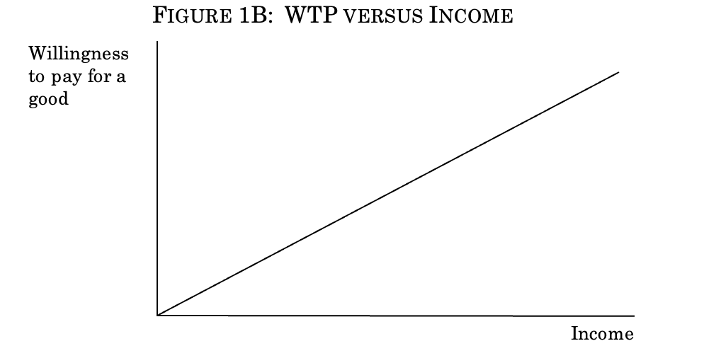
Figure 1 provides a graphical representation that helps explain what drives these results. Figure 1A shows the relationship between an individual’s utility and income—a curve that flattens out as one’s income increases. This pollution example involves two types of individuals with different levels of income, each of whom receives the same utility gains from an improvement in environmental quality. But even if the two types of people have the same utility gains, quite different amounts in dollars are needed to achieve these same utility gains. The y-axis shows equal utility gains for the rich and the poor groups. With connecting dashed lines, the figure then shows on the x-axis the dollar gains that would achieve those utility gains for each group. Because of the declining marginal utility of income (represented by the curved line), the amount of income it would take the rich to achieve the same utility gain is much larger. Dollars are “cheap” to the rich because they already have so many of them; thus, the rich need to receive a lot of dollars for a given utility gain. And this is precisely what drives the results in the example: the rich have a higher willingness to pay in dollar terms for the pollution reduction because dollars are cheap to them. As a result, efficiency analysis allocates the pollution reduction to the rich because, as Figure 1B shows, the willingness to pay for an allocation of goods goes up with income. The Appendix produces parallel figures for the neutral and poor-biased cases.

Figure 1:  Relationships for Rich-Biased Policy

Figure 1A:  Utility versus Income

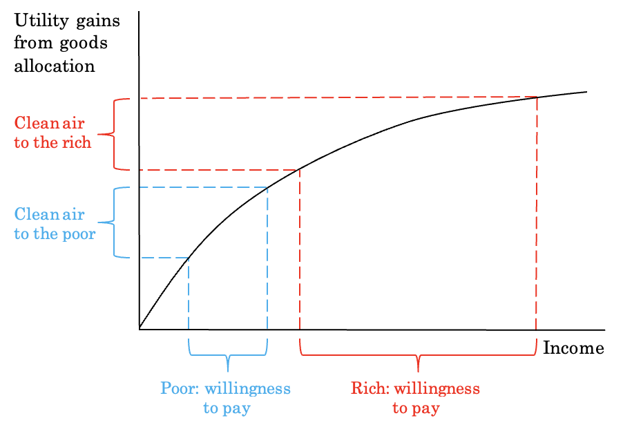
Figure 1B:  WTP versus Income

Again, nothing in this Article hinges on anything about utility functions. All we need to know is that empirically the rich tend to be willing to spend more than the poor on goods, which is why they in fact spend more. It is intuitive why they spend more: they have more money to spend. It could also be the case that they have different preferences or are able to borrow more easily or for a host of other differences. But what matters for efficiency analysis is the empirical difference in willingness to pay. Nevertheless, understanding the phenomenon in utility terms may ease interpretation of the prevalence and severity of the “rich get richer” principle.

IV. Examples of Efficient Rich-Biased Policies in Practice

To be influential, efficiency analysis need not explicitly be the decision-making rule that leads to a given policy outcome. Nevertheless, to help further concretize the ideas in this Article, this Part sketches a couple of the circumstances in which efficiency analysis is used explicitly in the law—particularly in rich-biased contexts because the business contexts in which neutral rules predominate are relatively straightforward. This Part first turns to federal regulatory cost-benefit analysis. It then describes how torts use efficiency analysis.

A. Federal Regulatory Cost-Benefit Analysis

Arguably the most prominent use of efficiency analysis by government actors is that by federal government administrative agencies, as required by executive orders originally dating to the 1980s and maintained by all presidents since then.110 According to federal guidance documents, federal regulatory analysis uses “benefit-cost analysis [to] provide[ ] decision makers with a clear indication of the most efficient alternative, that is, the alternative that generates the largest net benefits to society.”111 The potential for perverse distributive impacts is most stark when the analysis directly treats rich and poor people differently.112 For example, if the torts example used in Part III involving pollution affecting health outcomes were a federal regulatory proceeding, then the same distributional consequences would arise: a greater likelihood of pollution (without compensation) in poor neighborhoods than in rich ones. Sometimes, agencies use population averages of willingness to pay instead of disaggregating willingness to pay by the population affected so that rich and poor people are treated similarly.113 But sometimes they use different willingness to pay values for different income groups.114 And furthermore, Office of Management and Budget guidance suggests that agencies should use different values for different groups—for example, implementing different policies in different geographies due to differential benefits, presumably including some differential willingness to pay based on income.115 Moreover, at least one past top administrator of federal regulations (and prominent law professor), Cass Sunstein, has explicitly argued for using differential amounts of willingness to pay by income.116 This Section describes how transportation funding by federal agencies creates rich-biased rules.

In particular, the procedure for allocating Department of Transportation (DOT) funds affects how much it spends on modes of transportation that tend to be used by rich versus poor people. For calculating the benefits of transportation improvements, a key ingredient is the value of time saved in transportation as a result of the improvement. The DOT publishes a yearly memorandum on the Value of Time Travel Savings (VTTS) that adopts a higher VTTS for air and high-speed rail travel than for other surface modes of transportation for intercity travel, explicitly because the users of air and high-speed rail are richer than those of other surface modes of transportation.117 The memo explains that, “Since these modes charge higher fares to travelers who place a greater value on time saving, it is reasonable to derive a distinct VTTS from the higher incomes of their passengers.”118 DOT guidance adds that “[t]he value of travel time is a critical factor in evaluating the benefits of transportation infrastructure investment and rulemaking initiatives,” including competitive grant programs for infrastructure investment.119

This guidance affects the allocation of funds between transportation that rich people versus poor people tend to use. For example, every application for one of those competitive grant programs, the Transportation Investment Generating Economic Recovery (TIGER) program, must include a cost-benefit analysis.120 DOT guidance on preparing these applications instructs applicants to use the DOT’s VTTS.121 Thus, in funding TIGER grants,122 DOT relies on a higher VTTS number for airport projects (which are more likely to be used by the rich) than for bus projects (which are more likely to be used by the poor).123

As a result, because the monetary benefits of saving an hour of time for a rich person tend to be higher than the monetary benefits of saving an hour of time for a poor person, spending on transportation will be rich-biased, resulting in a bias in favor of more spending for the rich than for the poor for a given reduction in travel time.124 Thus, federal transportation spending has a built-in procedure that will tend to transfer more of a legal entitlement (transportation spending) to the rich, helping shorten their commutes, disproportionately easing their leisure travel, and disproportionately making them more productive.125

B. Torts

The primary example earlier in this Article concerned a tort against a polluter; it described the efficient duty of care required to establish the negligence standard, the threshold that, if exceeded, leads the polluter to pay damages.126 The Hand formula, which drove the determination of the negligence standard, is reflected in tort law. Indeed, the recent Restatement (Third) of Torts moved in the direction of focusing on the type of efficiency-oriented cost-benefit analysis described here,127 attracting some criticism for ignoring equity.128 The Restatement explicitly says that its “test can also be called a ‘cost-benefit test,’ in which ‘cost’ signifies the cost of precautions and the ‘benefit’ is the reduction in risk those precautions would achieve.”129 In estimating those costs and benefits, scholars see the Restatement as using the kind of efficiency analysis described in this Article.130 Of course, typically juries decide whether a duty of care has been met—and the extent to which juries are given instructions conforming with the Restatement is unclear (some suspect that it is infrequent131 ), but the efficiency-oriented Hand formula, with the distributional consequences described earlier, is clearly used at least sometimes.132

Efficiency analysis is apparent in other aspects of torts as well, particularly economic damages. In particular, workers are typically eligible for compensation for lost wages resulting from tortious behavior.133 Higher-income workers have higher wages and, thus, de facto have a larger legal entitlement. For example, consider a dangerous driver driving in a rich neighborhood versus a poor neighborhood. Drivers responding to incentives would expect to pay more if they cause an injury in the rich neighborhood than in the poor neighborhood. They may thus drive more dangerously in the poor neighborhood, increasing the likelihood of an accident there, thereby reducing the legal entitlement of poor groups to safe traffic conditions.134 But this is efficient: the rich are willing to pay more for not being injured than the poor are.

The purpose of this Article is not to lay out the broad spectrum of policy when efficient rules are adopted in ways that could lead to rich-biased rules. That is an important project, but one for another day. The purpose of this Part is merely to illustrate the concept with real-world examples—and to begin alluding to when efficient rules may be viewed as problematic, the issue that the next Part takes up.

V. Policy Implications

This Article is primarily descriptive, showing how different types of policies have different distributional implications. Nevertheless, this Part sketches potential policy implications of debiasing efficiency analysis, providing guidance on when and why to consider distributive consequences in economic policymaking and when to consider not adopting efficient policies if one has a goal of not redistributing toward the rich.

This Part takes “fairness” as a normative goal of institutions like courts and administrative agencies—in particular, not systematically distributing more legal entitlements to the rich or to the poor without compensating transfers. One could view this goal as a key attribute of the legitimacy of these institutions,135 as a requirement of Rawlsian fairness,136 as a libertarian goal of the government not picking and choosing policy winners, 137 or as a component of “folk justice.”138 Alternatively, one could view this kind of fairness as an instrumental feature of welfare; for example, as Part III.F shows, if both the rich and the poor suffer more in welfare terms as pollution increases, then it is welfare-enhancing to spread out the pollution between the rich and the poor rather than focus the pollution on the poor.139 However, because of the broad normative disagreement about the role of social welfare and redistribution in different ethical theories, this Article focuses on fairness, so defined. For example, some believe that, if welfare is the goal, federal agencies should redistribute toward the poor.140 On the other hand, while many may not want courts or administrative agencies distributing more legal entitlements to the rich than the poor because of efficiency analysis, they also may not want them redistributing to the poor either.

As a result, this Article adopts a fairly minimalist standard of fairness between the rich and poor in distributing legal entitlements while still taking advantage of opportunities that make all groups better off. To those unconcerned about the government distributing more legal entitlements to the rich than to the poor without the rich paying for them, the Article’s descriptive contribution stands even without these normative implications. But these implications are essential to those who hold any of the broad range of normative commitments suggesting that systematically distributing more to the rich is problematic.

One possible response to this Article’s analysis is to ignore efficiency altogether given its bias against the poor. That approach seems unwise. Efficiency creates economic surplus—growing the size of the economic pie—that, in principle, can be redistributed to make everyone better off. For example, the government could invest more in airports (largely benefitting the rich) and less in buses (largely benefitting the poor), and then increase transfers to the poor. Doing so could be efficient because of the rich’s relatively high willingness to pay for airport improvements. Furthermore, in neutral cases, in which the distributional impacts may even out, ignoring efficiency could mean ignoring opportunities to make everyone better off.

Rather, this Article suggests a different approach: taking guidance from legal context. This Article’s analysis suggests a two-part inquiry for efficient policies, as laid out in the flow chart in Figure 2. If two conditions hold and one does not want to distribute more to the rich than to the poor—while still taking opportunities to make all groups better off—then efficient legal rules should be modified to be inefficient and make equal allocations to the rich and poor. That is, if one has a goal of not redistributing toward the rich in judicial, administrative, or even legislative rulemaking, the results imply that different policies should be adopted depending on the legal context. The analysis, of course, applies only to efficient rules. Lots of adopted policies are not efficient, with a variety of distributional consequences, but they are not implicated by the analysis here.

Figure 2:  When Efficient Policies Should Be Modified to Treat Rich and Poor Alike

 

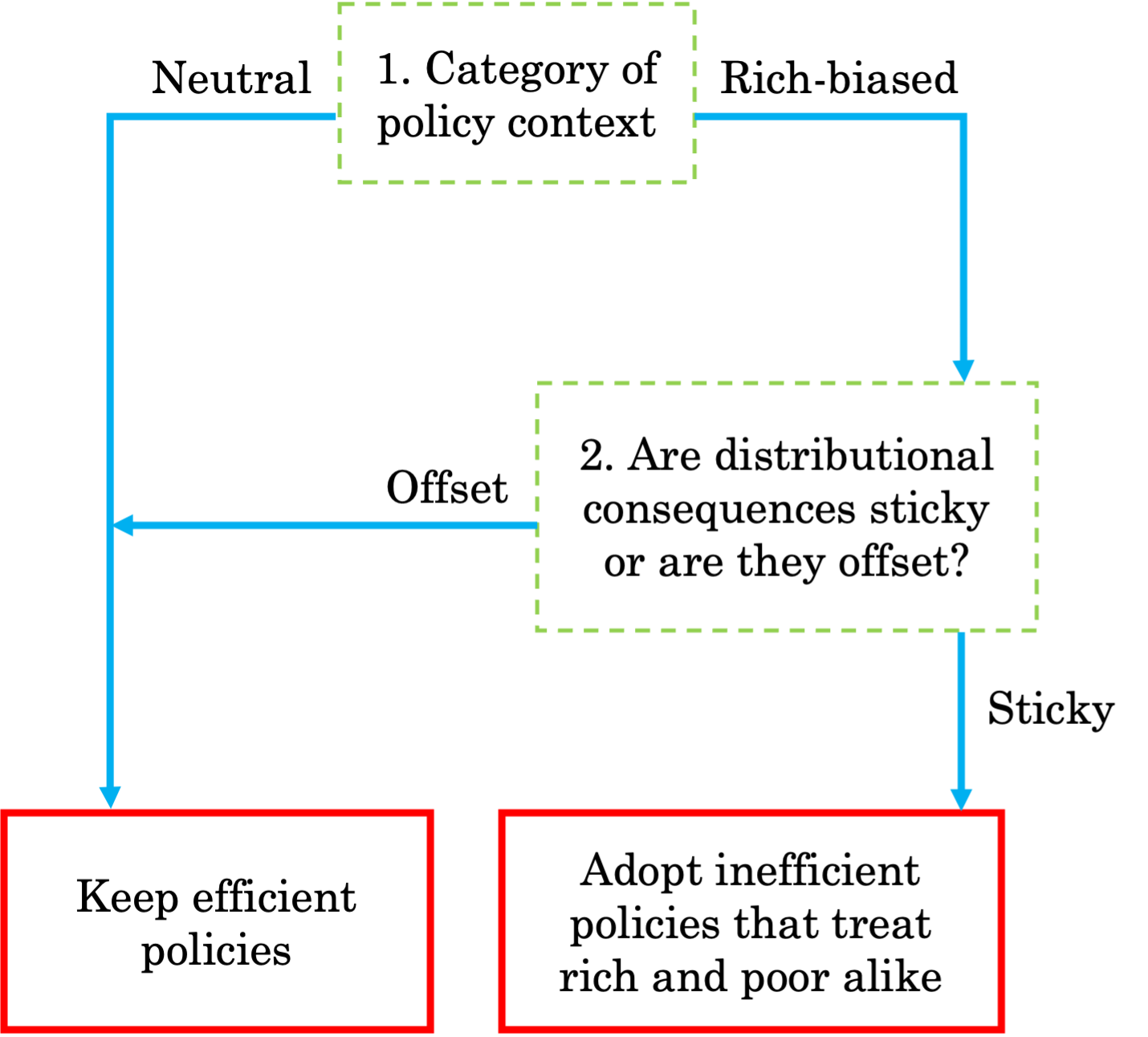
The approach begins with a threshold bifurcation: Is the context one that is likely to lead to a rich-biased rule? If so, then the distributional concerns that this Article describes will arise. For neutral policies like those resulting from changing business profitability, policymakers could hold different views on the necessity of compensating losers on a policy-by-policy basis, but there is a supportable argument that policy impacts could even out over a large number of policies: there is no inherent bias. Any given policy may benefit the rich or the poor. But the rich and poor “count” equally because each has the same willingness to pay for $1. So efficient neutral policies may tend to make all income groups richer.

For rich-biased policies, in contrast, the notion that distributional impacts will even out is not plausible. Rather, there is an inherent legal entitlement bias. If one holds the view that policy should not distribute more legal entitlements to the rich than to the poor without making the rich pay, then this result should cause concern. Even rich-biased policies with small distributional stakes risk perverse impacts: lots of small biased policies can add up to a lot of bias in aggregate.141 These distributional impacts justify inefficient policies that treat rich and poor alike if another condition holds.142

Second, are the policy’s distributional consequences likely to be offset or sticky? Or something in between? As Part I describes, inertia and interest groups could contribute to a lack of offset. The lower the probability of distributional offset, the greater the risk of perverse distributional consequences. While it is beyond the scope of this Article to delve into this issue, several factors could contribute to the likelihood of offset.143

First, the institution adopting the policy can matter. In general, legislatures, with their taxing power and greater perceived democratic legitimacy, can more easily adjust policies to address distributional concerns. In contrast, administrative agencies and courts are less able to offset distributional consequences, making it more likely that perverse distributional consequences will stick. Of course, other institutions may act to offset those distributional consequences; for example, an administrative agency may enact a rich-biased rule with substantial distributional consequences, and the legislature can offset those consequences. But the fact that it would be difficult for the administrative agency itself to offset them probably makes it less likely that they will be offset than in the case of a legislature.

Second, the salience of the change may matter. Large, salient changes may be more likely to attract attention and be offset, while small changes that fly under the radar may be less likely to attract attention. For example, the 2010 Patient Protection and Affordable Care Act144 was a large and salient form of redistribution—and also helped generate a backlash that put Republicans in power.145

Third, offsets that comply with voters’ moral intuitions may be more likely to be achieved. For example, recent empirical evidence suggests that many individuals do not view taxes primarily as a means of redistribution.146 As a result, offsets that would require large transfers through the tax code may be politically difficult to achieve. On the other hand, offsets that can be accomplished by, say, directly compensating the losers of government policy or through expanded social insurance may be more palatable and thus more likely to happen.147

Fourth, when the government has the tools to offset distributional consequences, offset is presumably more likely. For example, suppose that a state court enacts a change with distributional consequences. States that have progressive income taxes that impose different rates on the rich and the poor may be more likely to be able to offset those consequences because they have a good tool to do so. Specifically, they could change the progressivity of their state income taxes compared to states that have a flat state income tax rate and thus do not have such a tool.148

Finally, as Part I discusses, groups that are better able to organize may be more likely to achieve their distributional objectives, as described by the public choice school of economics.149 Thus, when the relative losers from a policy change are disbursed, politically weak, and unorganized, offset may be less likely.

In any case, an individualized determination based on the actual legal context—including the institution and policy involved—is required here. For example, a rich-biased efficient policy on transportation spending adopted by federal regulation in the Obama Administration was presumably more likely to be offset through congressional action in 2009–2010, when Democrats relatively supportive of redistribution to the poor controlled Congress, than in 2011–2016, when Republicans controlled the House of Representatives.150 Of course, offset need not be immediate—but as noted earlier, the distributional consequences in the short and medium run may matter more than those in the long run.151

If policies reach the bottom right of the flow chart—that is, if they are (1) efficient, rich-biased policies with (2) a low probability of offset—then they deserve different treatment. With this set of policies, for those with a broad set of normative commitments, this Article offers an important reason to consider adopting less efficient legal rules that are less biased against the poor and that instead treat the rich and the poor the same way.

Concretely, under this reasoning, after Republicans opposed to more transfers to the poor took control of the House of Representatives in 2011, the Obama Administration should have issued guidance that had the same value of time figure for the rich and the poor when calculating the value of transportation improvements. Instead, in the face of persistently high income inequality that it professed to find problematic152 and little prospect of increased transfers to the poor,153 the Administration used guidance that contained a systematic bias toward transportation improvements benefitting the rich over those benefitting the poor.

Taking other examples discussed earlier in this Article, this framework could also mean:

• Following the same liability standard for polluting on poor and rich individuals;
• Spending the same amount on research and development for a given reduction in diseases that affect rich and poor people;
• Spending the same amount for a given improvement in road safety, the ease of voting, or speed of commuting for the rich and the poor;
• Spending the same amount for a given reduction in crime for the rich and the poor;
• Building similar parks in rich and poor neighborhoods.

These steps treat the rich and the poor in similar ways across various rich-biased policy areas. For example, as Professors Matthew Adler and Eric Posner have described, administrative rulemakers could adjust parties’ measured willingness to pay to remove the effect of income, thus “launder[ing]” parties’ preferences.154 How to do so will again depend on legal context, and it is beyond the scope of this Article to work out how to do so in any given circumstance. But it is fair to say, given the centrality of efficiency to policymaking and the frequency and severity of the bias, that the consequences would be profound.

Finally, to be clear, for policies that do not satisfy both conditions, this Article does not claim that there should be no modification from the efficient policy. For example, to correct perceived inequalities in existing policy, a committed redistributionist may want to modify efficient neutral rules, especially those that distribute more to the rich than to the poor, to promote a more egalitarian distribution of income.155 Nor is there necessarily any moral difference between two rules—one neutral and the other rich-biased—with the same distributional consequences. Others should explore this. There is, however, a difference in whether there is a systematic bias in how efficient rules will allocate entitlements. And this Article has adopted a weaker standard with wide acceptance across those with many political commitments: that the government should not systematically distribute more to the rich than to the poor solely because of the rich’s greater wealth without compensating policies for the poor.

VI. Responding to Potential Critiques

A. Considering Economic Growth

One potential criticism of the analysis is that it seems static—that is, it considers efficiency only at a point in time rather than considering impacts on economic growth.156 The concern here is that the pursuit of efficiency, even if it increases inequality, also spurs growth by increasing, for example, the accumulation of capital and innovation, ultimately leading to higher income for everyone. In its analysis, this Article engages in the standard practice of not considering growth effects, and the goal in this Article is not to question that standard practice. Nevertheless, this Section touches on a few reasons that this Article’s analysis stands even when considering growth.

The first is the most important and the most basic: with a simple redefinition of the question, the same underlying logic applies and the same broad conclusions are true—efficient policies tend to be rich-biased. Instead of thinking about the policy question as pertaining to one point in time, think about policies across, say, a hundred-year period, including economic growth over that period. An efficient rich-biased policy that creates a given amount of surplus over a hundred-year period will still allocate a larger amount of the legal entitlement to the rich than to the poor because the rich at any point in time are willing to pay more.

There are two other responses as well. First, even ignoring such a redefinition, to benefit the poor, the benefits have to reach the poor—and as much recent research has shown, for the most part, that has not happened in decades through either rising wages or changing economic policies.157 Second, growing evidence suggests that inequality itself reduces economic growth, potentially making everyone worse off, as a recent International Monetary Fund report argued, for example.158

More broadly, the division between neutral and rich-biased policies developed in this Article raises questions about the extent to which a pursuit of efficiency really promotes growth. Neutral rules maximize dollars. As a result, the efficient rule produces an economy with more investable capital for use on new machines and innovations, increasing growth.159 In the torts example above, as a result of the efficient liability rule, the economy becomes $5,000 more productive. (That is, the economy is able to produce the same goods and services at a cost $5,000 less than without the efficient rule because the rule induces the factory to install the scrubbers at a cost of $5,000 instead of making the laundromat install the air purifier for $10,000.) Thus, businesses have $5,000 more to spend on growth-inducing investments. To those who think that dynamic growth is very important to lifting all boats in the long run and that capital accumulating aids in growth, this neutral legal rule achieves that goal.

However, the results are quite different for the rich-biased rule. Rich-biased rules maximize willingness to pay units, not dollars. In a rich-biased rule like that in the torts example, there is no increase in investable capital or other increase in innovation when allocating the clean air to the rich homeowners but not the poor homeowners. The factory’s profits decrease if it purchases the scrubbers, thereby reducing its investable capital, but there is no difference between the cases of the rich and poor homeowners because the homeowners themselves are just accumulating WTPs and not dollars through the efficient legal rule. Thus, in allocating clean air to the rich homeowners but not the poor homeowners, the economy is richer in WTPs, but there is no increase in investable capital that could have dynamic growth effects, further undercutting the value of rich-biased rules to those who focus on the growth-inducing effects of focusing on efficient legal rules.

B. Adding Complexity to Policymaking

One may argue that this analysis misses a host of potential complicating factors. For example, returning to the rich-biased case of the homeowner and the factory, consider how the factory’s decision to pollute might affect gentrification, such as whether new people migrate into the neighborhood, crime goes up or down, or a host of other factors. Those are good points, and any full analysis would want to consider them. But that’s not a criticism of anything that this Article suggests; rather, it is a criticism of efficiency analysis itself. If those factors are easily incorporated into WTP calculations, then they presumably will be. If not, then they may not be—but the point does not blunt the force of this Article’s critique.

But another set of concerns this Article raises does add complexity to the analysis. In particular, the policy response section suggests that analysis and policymaking should take into account contextual factors, including the likelihood of distributional offset. Allowing the possibility of different political responses into the analysis would add complexity, versus merely assuming—regardless of context—that all distributional consequences are offset. Readers will need to decide for themselves between the merits of the possibilities: (1) adopting possibly wrong assumptions in the name of simplicity—with the potential distributional consequences this Article describes—versus (2) adopting more flexible assumptions about politics that may be more realistic, adding complexity but also reducing the risk of perverse distributional consequences.

Conclusion: Law and Economics in an Age of Inequality

When then-Professor Richard Posner published the efficiency-oriented Economic Analysis of the Law in 1972, law and economics scholar Professor A. Mitchell Polinsky called the book a “potentially defective product” in that “even a valuable product is subject to misuse if proper instructions are not included.”160 In particular, the distributive consequences of policies had to be considered.161 Despite Polinsky’s warning, economic analysis of the law has long been guided by the assumption that the distributive consequences of policies do not matter because taxes should respond to take care of distributive considerations. But there is little evidence that taxes in fact do respond. This Article draws out the distributive implications of adopting efficient policies when other policies do not offset those distributional consequences.

This Article shows that, under many circumstances, efficient policies are not merely neutral with respect to the distribution of income. Rather, efficient policies systematically tend to distribute legal entitlements to the rich, exacerbating inequality. Especially given the widespread concern over rising income inequality, it is time to consider adopting policies that reduce efficiency but have fairer distributional outcomes, at least in some circumstances. The necessary analysis may be more difficult, but—lacking evidence that the perverse consequences of efficient rich-biased policies are offset—such policies are worth pursuing in the appropriate contexts.

How policymakers should respond is a longer-term project. One can imagine two extremes: (1) always adopting efficient policies and (2) ignoring efficiency altogether. Both have unappealing features. Without offsetting policies, always adopting efficient policies will have a systematic bias against the poor. On the other hand, ignoring efficiency altogether means missing out on opportunities to make all groups better off. Efficient neutral policies have distributional impacts that may even out and make everyone better off. And if there are some taxes and transfers, then considering willingness to pay driven by income allows the combination of efficient policies with taxes and transfers to make everyone better off.

Rather, if policymakers consider distributional consequences with a goal of being fairer, this Article suggests the importance of considering context in deciding whether to deviate from the efficient rule. First, is the legal context one of neutrality or rich bias? Because neutral policies have distributional consequences that may even out in the long term while rich-biased policies do not, the case for deviating from the efficient rule is stronger for rich-biased policies. And second, are the distributional consequences likely to be offset or be sticky? This second question is one of political economy, a topic that is typically absent in economic analysis in lieu of an implicit political economy assumption that the consequences are offset. For efficient, rich-biased rules with distributional consequences that are sticky, a broad range of political commitments suggest that policymakers should adopt explicitly inefficient rules that treat the rich and the poor alike.

These contextual elements powerfully motivate avenues of future scholarly research. A first implication is empirical in nature: When is distributional offset likely to happen and when is it not? The more promising the prospects for offset, the more traditional efficiency analysis is appropriate. More broadly, a second empirical task is determining which policies can benefit the poor the most while causing the least loss in efficiency.

Likewise, the results raise the urgency of actually implementing offsetting taxes and transfers, which can make everyone better off in concert with efficient policies. Failing increased offset, though, the results suggest a greater scope for law and economics analysis that trades off equity and efficiency to complement existing efficiency-minded law and economics analysis, and for more policy that puts the rich and poor on equal footing rather than making the rich richer.

Appendix

This Appendix first presents the technical definition of Kaldor-Hicks efficiency in Section A. Section B then presents the technical definition of “legal entitlement neutrality.” Section C presents the result that a simple formula can be used to determine if a given utility function produces rich-biased, neutral, or poor-biased legal rules. It then explains the intuition for the result. Section D maps this Article’s categorization onto the conventional economics definitions of “normal” and “inferior” goods. Section E shows utility functions that correspond to each type of policy and explains them graphically. Section F shows the math behind Part III.F’s example of tradable pollution permits.

A. Technical Definition of Efficiency

The following notation defines K-H efficiency. There are I  individuals indexed by i . Suppose that there is some thing x that the government is allocating through public policy to individuals such that individual i  receives quantity xi≥0  with ixi≤X .162 K-H efficiency asks which of these allocations creates the greatest amount of aggregate social surplus, denoted for each individual by sixi.  K-H efficiency adds up the surplus for each individual and chooses the set of allocations with the highest sum; that is, it chooses the policy that satisfies maxx1, . . . ,xIisi(xi) .

Surplus measures how much a policy increases the expenditure function, denoted  eiv , which measures the smallest amount that an individual needs to spend to achieve utility level v . In other words, the expenditure function, and thus surplus, is a measure of how much people are willing to pay for a policy change. More precisely, surplus compares the expenditure function evaluated at the utility under the alternative policy vi1  (with given allocation xi ) with the expenditure function evaluated at the status quo utility level vi0 , or si= eivi1 - eivi0 . For example, suppose that: (1) under the status quo policy, an individual achieves a utility level of 13 and spends $100 to achieve; (2) she would achieve a utility level of 15 with a new government policy allocation xi ; and (3) it would take $150 of spending to achieve a utility level of 15 under the status quo policy. Then  ei13=$100 ,  ei15= $150 , and sixi=$50. Surplus thus measures how the expenditure function changes under different possible policies. It measures the amount that individual i  would have to pay or be paid to make her indifferent between the status quo and the alternative policy. In this example, the individual would be willing to pay $50 to shift to the new policy. This amount is unique to each individual, as determined by her utility function and income.

B. Legal Entitlement Neutrality

Legal entitlement neutrality means that:

where (as described above) s  is surplus, x  is some policy variable (conceptualized here as an entirely government-provided good or service), and c  is one’s consumption or income (which are equivalent and thus interchangeable in this one-period model because people consume all their income) such that utility u_i=u(c_i,x_i) . The interpretation of the condition is that, as income c changes, the extent to which an increase in policy variable x increases surplus s (∂s/∂x)  does not change. That is the condition for not changing the allocation of legal entitlements as people get richer because increased surplus is what drives larger allocations in efficiency analysis. Note a couple of restrictions with this setup: there are only two goods, and transaction costs are not explicitly modeled.

If providing good or service x provides more surplus s as one’s income c increases, then it is a rich-biased policy: because the rich are willing to pay more for it, efficiency-oriented analysis will endow well-off individuals with more of it than poor individuals. For rich-biased policies, ((∂^2)s)/∂x∂c>0.

In contrast, if the poor are willing to pay more for the good, so that surplus for the provision of x increases as income decreases, then the good is poor-biased. For poor-biased policies, ((∂^2)s)/∂x∂c<0.

In between are neutral goods, for which income does not impact the surplus from provision of the good. That is, ((∂^2)s)/∂x∂c=0.

C. Relation of Legal Entitlement Neutrality to Utility Functions: Main Results

This Section of the Appendix defines legal entitlement neutrality in terms of utility functions. As noted earlier, the determination of legal entitlement neutrality is in principle measurable empirically without reference to utility functions. Nevertheless, understanding from a utility framework what drives whether a policy is legal entitlement neutral may be helpful for those who think in such terms. In particular, this setup yields the following result:

Result 1: A policy is rich-biased if and only if:

 

The proof is below; I focus here on intuition. The formula compares two things: (1) how more consumption c changes the marginal utility of good x(((∂^2)u)/∂c∂x)  with (2) the slope of the marginal utility of consumption ((∂^2)u)/∂c^2 , or how more consumption changes the marginal utility of consumption, multiplied by the ratio of the marginal utility of good x divided by the marginal utility of consumption to normalize utility.163 We know that, under typical assumptions, the first term ((∂^2)u)/∂c∂x  has an unclear sign, but the second set of terms (((∂^2)u)/∂c^2)∙((∂u/∂x)/(∂u/∂c))  is negative because ((∂^2)u)/∂c^2<0  by the declining marginal utility of income and ∂u/∂x>0  and ∂u/∂c>0  by nonsatiation.

Thus, the formula boils down to a simple comparison: whether, as an individual’s consumption increases, the marginal utility from policy x decreases more rapidly than that of income (scaled by the ratio of marginal utility for policy x and consumption). If the marginal utility of policy x  decreases less rapidly than the utility of income, then the good is rich-biased—for example, if the utility of the good (say, clean air) stays constant with income ((∂^2)u)/∂x∂c=0  and there is a declining marginal utility of income ((∂^2)u)/∂c^2<0 . If the inequality goes the other way, the good is poor-biased. And if the two terms are equal, the good is neutral. In other words, goods that poor people really want—that they get so much utility from that they are willing to pay more for them than rich people, despite their greater poverty—are poor-biased. Otherwise, goods are rich-biased or neutral.

The intuition for the result is as follows: efficiency-based legal entitlement allocations are based on willingness to pay. Suppose for simplicity that the utility of something stays constant with income (for example, both rich and poor people may value clean air the same amount in utility terms)—in other words, the first term of the formula in Result 1 equals 0. Then the willingness to pay for something increases with income as long as the utility from yet an extra dollar of consumption goes down as income increases—in other words, as long as there is a declining marginal utility of consumption (that is, the second term in Result 1 is negative). But other times, one’s utility from having something does not stay constant with income and instead declines with income. In those cases, when the utility of having the thing declines rapidly enough, willingness to pay can stay constant or even decline with income.

Overall, then, there are three factors inclining a good to be rich-biased, corresponding to the three terms in the formula in Result 1. First, as one would intuitively expect, when income has a more positive effect on the marginal utility of good x, good x is more likely to be rich-biased. Second, when the marginal utility of consumption is diminishing very rapidly (that is, it is strongly negative), the policy is more likely to be rich-biased because it will take a large money transfer to make up for the utility gains from the policy. Third, when there is a high ratio of utility gains from the policy x versus consumption c, the good is more likely to be rich-biased. Again, this is intuitive because it will take more money to compensate for the gain of x if the marginal utility of income is lower relative to the marginal utility of the good x.

1. Derivation of utility result.

The goal of the result is to sign ((∂^2)s)/∂x∂c  as a function of utilities. As noted above, there are two goods, policy variable x and numeraire consumption good c such that utility u_i=u(c_i,x_i). Suppose that the policy variable x is entirely government provided, so that endowment y=c (because the only thing to spend money on is c). As a result, we can discuss the marginal utility of consumption c and the marginal utility of income y equivalently.164 Thus, ((∂^2)s)/∂y∂c=((∂^2)s)/∂x∂c. Suppress taxes because their presence adds terms without adding insight. Also, suppress prices because this Article has only a government-provided good and a numeraire good.

To start, recall that s  is defined as follows: s=e(v_i^1) - ei(v_i^0) . But we know that v_i^1=u(c_i,x_1) and v_i^0=u(c_i,x_0). That is, we can replace utility achieved v with the utility function u. Furthermore, because the equivalent variation is equal to the change in the value of the expenditure function accompanying a policy change,165 equivalent variation (or “surplus,” s ) can be replaced with the expenditure function e . Making that substitution and working out the derivative yields:

Thus:

 

Turning away from this line of argument for a moment, we know from price theory that e(v)=e(u(c))=c  because individuals allocate their entire budget to a single numeraire good with a price of 1. That is, total expenditure will equal one’s endowment, which in this case is equal to c. Totally differentiating e(u(c,x))=c  with respect to c  yields:

 

Totally differentiating with respect to c  a second time yields:

Rearranging gives:

Substituting (2) into (1) gives (after simplification):

As a result, assuming that ∂u∂c>0,  (that is, utility is increasing in consumption), the sign of ((∂^2)s)/∂x∂c  is the sign of

This proves the result.

D. Legal Entitlement Neutrality and Normal and Inferior Goods

This setup also produces the following result:

Result 2: Rich-biased goods are “normal” goods, in which demand for the good increases with income; poor-biased goods are “inferior” goods, in which demand for the good decreases with income.

I begin by introducing the notation that p  is the price in a hypothetical market for good x . The maximization problem is then the same as before:

This implies that we can rewrite the utility function as u(x,I-px) .

The first-order condition is

This condition holds at the utility-maximizing point, (x*,c*)

Taking the derivative of (6) with respect to I  yields

Note that

 

Substituting (8) into (7),

 

Finally, by (5), I can rewrite (9) as

Note that the denominator is the second-order condition, which by the normal regularity conditions is negative.

Thus, by (4), (∂x*)/∂I>0  (that is, x is a normal good) if and only if x  is rich-biased, (∂x*)/∂I<0  (that is x is an inferior good) if and only if x is poor-biased, and (∂x*)/∂I=0  if and only if x is a neutral good.

E. Legal Entitlement Neutrality: Graphical and Utility Representations

This Section of the Appendix presents two additional ways of helping to understand legal entitlement neutrality. The first way is through graphical demonstrations of the forms of bias, complementing the portion in the main body of the text on rich bias. The second way is an exploration of utility functions, which helps show why poor-biased policies are rare and rich-biased policies are common. It turns out that utility functions that economists are familiar with tend to be rich-biased. Economists use these utility functions not only because they are relatively convenient but also because they conform with consumer behavior: for example, declining willingness to pay as quantities increase and a preference for diversity. This Section of the Appendix shows which utility functions correspond to which type of policy and shows graphically why they exhibit their type of bias.

1. Rich-biased policies.

Many of the most common utility functions are rich-biased. Consider the following examples.

Separable utility functions: For any separable utility function (in which u=f(c)+f(x)), ((∂^2)u)/∂c∂x=0 . As a result, the sign of (3) is positive, and thus there is prorich bias.

Cobb-Douglas: For utility functions of the form u=A(c^α)(x^(1-α)) , for 0<α<1  and A>0 , we know that policies are rich-biased because ((∂^2)u)/∂c∂x=Aα(1-α)(c^(α-1))x^(-α)>0  because every term is positive. Thus, equation (3) is positive, and this utility function is rich-biased.

Constant Elasticity of Substitution: Constant elasticity of substitution utility functions of the form u=(αc^r+(1-α)x^r)^(1/r) , for 0<α<1  and -∞<r<1 . For these, we know (((∂^2)u)/∂c∂x)-((∂^2)u)/∂c^2∙(∂u/∂x)(∂u/∂c)=(1-r)(1-α)(αc^r+(1-α)x^r)^(1/r-1)x^(r-1)c^(-1)>0.166 We know that this result is positive because every term is positive as a result of α,r<1 . So equation (3) is positive, and these functions are rich-biased.

An example rich-biased utility function for the homeowners in the torts example in the main body of the text is u=logc+logx , where c is consumption and x is a clean environment. That is, there is a declining marginal utility of consumption, and everyone gets the same (declining) utility from a clean environment.

2. Neutral policies.

Determining the sign of (3) is trivially easy when the “good” is the same thing as the numeraire good, or money. Then c=x , and (3) reduces to

which meets the definition of a neutral policy.

An example neutral utility function for the laundromat owners in the torts example in the main body of the text is u=logc+x , where c is consumption and x consists of the profits that result from having cleaner air. Thus, the laundromat owners value the profits from their laundromats just like any other money that leads to consumption.

To understand the results graphically, recall Figure 1 on rich-biased policies in the main body of the text, which shows utility gains from a policy that are the same for the rich and the poor. Compare that figure to Figure 3, which has utility gains not from gaining a rich-biased good but rather from gaining dollars. Figure 3A compares the utility gains for a given dollar gain between the rich and the poor. Because of the declining marginal utility of income, a given dollar gain will result in a smaller utility gain to the rich than to the poor, as reflected on the y-axis. However, the same dollar gain will result in the exact same willingness to pay between the rich and the poor, as reflected on the x-axis. Thus, as shown in Figure 3B, for a given dollar gain (say, $100), the income of the person receiving the income does not vary the willingness of the person to pay for the dollar gain: a dollar is worth a dollar to everyone.

Figure 3:  Relationships for Neutral Policy

Figure 3A:  Utility versus Income

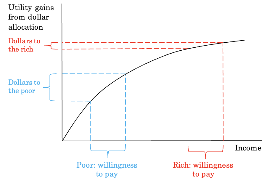
Figure 3B:  WTP versus Income

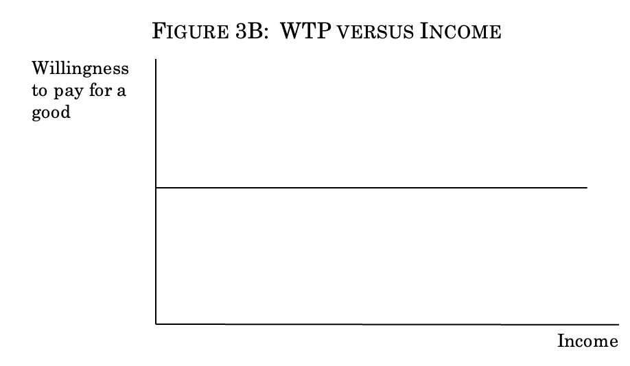
3. Poor-biased policies.

Take the utility function u=log(x-1/2)-2∙log(10-c), for x>1/2  and 0≤c<10 , which is a member of a class of utility functions for which x is an “inferior” good (for example, bus service) in which the poor demand a higher quantity of it than the rich do.167 Here, we know:168

((∂^2)u)/∂c∂x-((∂^2)u)/∂c^2∙(∂u/∂x)/(∂u/∂c)=0-1/(10-c)(x-0.5)<0

So this utility function is poor-biased.

One can think of poor-biased policies graphically as those for which there is such an enormous difference in the utility gained by a rich and a poor person that the difference overcomes the declining marginal utility of income—in other words, it overcomes the fact that it is a lot more expensive to pay off a rich person than a poor person in dollars for a given utility gain because of the declining marginal utility of consumption. Figure 4 shows this case. Because the utility gains to the rich are so much smaller than those to the poor on the y-axis of Figure 4A, the poor actually have a larger willingness to pay on the x-axis. The declining willingness to pay with income in Figure 4B results.

Figure 4:  Relationships for Poor-Biased Policy

Figure 4A:  Utility versus Income

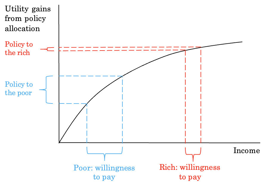
Figure 4B:  WTP versus Income

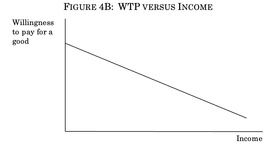
4. Intuition for the “rich get richer” principle.

The result here shows that the bias of the policy depends on the comparison of how utility changes with income and the marginal utility of income. The earlier figures portray this comparison by showing on the y-axis with brackets the different utility gains of rich and poor people for a policy change and then using the curve for the marginal utility of income to translate those utility gains from a policy change into a willingness to pay.

To see this graphically a different way, consider Figure 5, which beneath the axis shows who (the rich or the poor) gains more utility from a policy change and above the axis shows the direction of the bias. On the left half of the figure, the rich gain more utility than the poor: those policies are rich-biased, as the scale above the axis shows. In the middle (“Rich = poor”), utility gains are equal. At that point, the policy exhibits prorich bias. To the right of that point, the poor gain more utility than the rich, but the prorich bias continues until the utility gains from the policy decline at the same rate as the marginal utility of consumption declines, at which point the policy is neutral. It is only to the right of that point—a narrow portion of the overall spectrum—that there is propoor bias. The nature of efficiency is such that it tends to produce outcomes that favor the rich.

Figure 5: Bias and Utility Gains from Policy

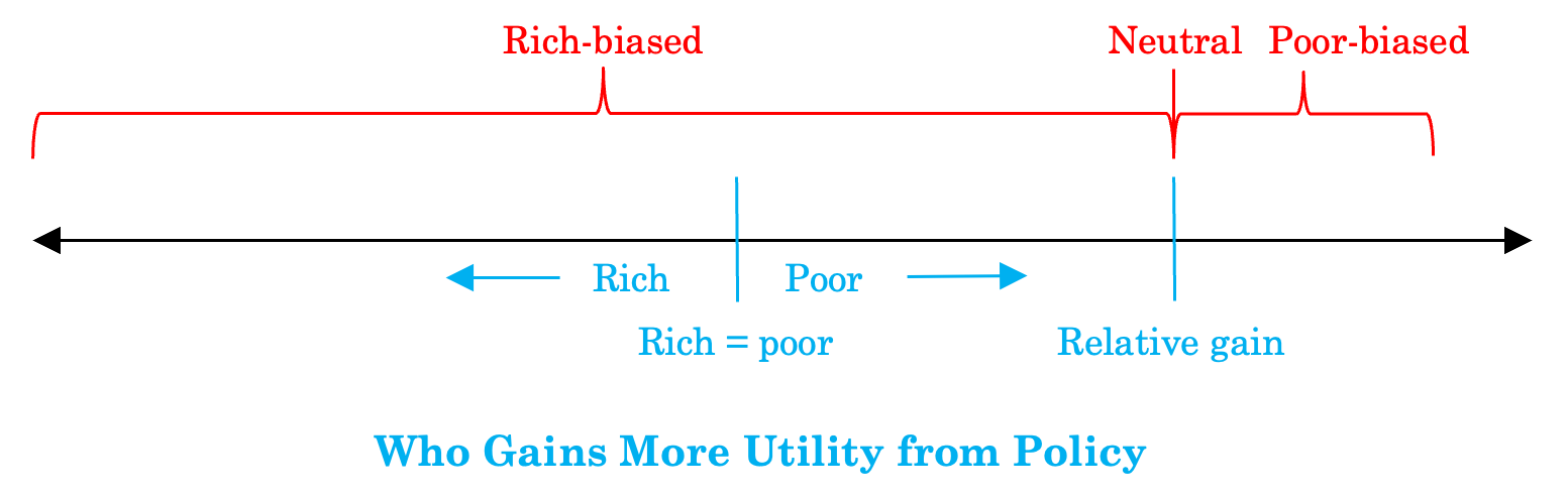
F. Math for Tradable Pollution Rights

Part III.F describes tradable pollution rights. This Section solves for the price with these tradable pollution rights.

1. Optimal allocation.

The poor maximize u_p=log(1+x_p)+logc_p  s.t. c_p= y_p+g(x(mean)_p-x_p), and the rich maximize u_r=log(1+x_r)+logc_r s.t. c_r= y_r+g(x(mean)_r-x_r) by choosing cleanliness units x_p and x_r, respectively, given price for cleanliness g, initial allocations of cleanliness x_p and x_r, and income allocations y_p and y_r. The social planner wants to choose x_p and x_r so as to maximize

There are ten units of cleanliness in total, so

The initial endowments are y_p=1  and y_r=9 .

To solve for the initial allocations, the final allocations, and the price of a unit of cleanliness, I first solve for the cleanliness demand curves of the rich and the poor. Rewriting the utility functions in terms of cleanliness yields u_p=log(1+x_p)+log(y_p+gx(mean)_p-gx_p) and u_r=log(1+x_r)+log(y_r+gx(mean)_r-gx_r). Taking the first-order conditions with respect to cleanliness gives the demand curves

Combining the demand curves (14–15), equation (12), and the social welfare function (11), we get SWF = log((y_p+gx(mean)_p+g)/2)g+log(y_p+gx(p)+g/2)+ log((y_r+g(10-xp)+ g2g+ logyr+g(10-xp)+ g)/2). Solving the first-order condition for xp  and substituting in the values of the endowments gives:

This implies that x(mean)_r= (5g-4)/g, x_r= (5+4g)/2g , and x_p= (5+4g)/2g . Combining the final allocations with equation (13) reveals that the price of cleanliness is g=5/6 . With this price we can solve for all other values. Thus, x(mean)_p= 49/5, x_r= 1/5, x_p= x_r= c_p= c_r=5 .

2. Even allocation with trading.

If the initial allocation of cleanliness is five for both rich and the poor, then substituting into the demand curves (14 and 15) along with the initial endowments gives

x_p= (1+4g)/2g  and x_r=(9+4g)/2g

Combining this with equation (13) gives that the price is again g=56  and the final allocations are x_p= 13/5 and x_r=37/5 .

• 1To simplify, assume for now that people do not move due to park construction so that no gentrification occurs. See discussion of issues like gentrification in Part VI.B.
• 2See, for example, Lisa Heinzerling, Quality Control: A Reply to Professor Sunstein, 102 Cal L Rev 1457, 1458 (2014) (“For more than three decades, executive orders governing White House regulatory review have specified cost-benefit analysis [another term for analysis of economic efficiency] as the normative framework for evaluating agency rules.”); Matthew D. Adler and Eric A. Posner, Rethinking Cost-Benefit Analysis, 109 Yale L J 165, 167 (1999) (“[Economic efficiency’s] popularity among agencies in the United States government has never been greater.”). For commonly used textbooks taking this view, see, for example, Richard A. Posner, Economic Analysis of Law 15–20 (Wolters Kluwer 9th ed 2014); Robert Cooter and Thomas Ulen, Law & Economics 7–8 (Addison-Wesley 6th ed 2012) (saying that the book “will focus on efficiency rather than distribution” in analyzing the law because of the availability of the tax system for redistribution); Steven Shavell, Foundations of Economic Analysis of Law 2–3 (Belknap 2004) (describing social welfare as the normative basis for analysis in law and economics, but then restricting attention to efficiency by excluding analysis on distribution).
• 3See Executive Order 12866 § 1 (1993), 3 CFR 638, 638–40 (requiring cost-benefit analysis in federal agencies); Regulatory Analysis, Circular A-4 *8 (Office of Management and Budget, Sept 17, 2003), archived at http://perma.cc/A4NA-R3P5 (“Where there are significant regional variations in benefits and/or costs, you should consider the possibility of setting different requirements for the different regions.”). See also Part IV.A (listing examples).
• 4See Richard A. Posner, The Ethical and Political Basis of the Efficiency Norm in Common Law Adjudication, 8 Hofstra L Rev 487, 502–07 (1980) (arguing that the common law is efficient and that this is normatively desirable). See also Part IV.B (listing examples).
• 5Email from Lawrence Mishel, former President of the Economic Policy Institute, to Zachary Liscow (Jan 3, 2018, 8:23 pm CST) (on file with author).
• 6See, for example, Richard O. Zerbe and Tyler A. Scott, (Almost) Everybody Wins: A True Pareto Justification for Practical Welfare Economics and Benefit-Cost Analysis, *25 (University of Washington School of Law Legal Studies Research Paper Series, 2014), archived at http://perma.cc/LJ5P-WRAR; Leslie Carbone and Jay Richards, The Economy Hits Home: What Makes the Economy Grow? (The Heritage Foundation, July 1, 2009), archived at http://perma.cc/8B7G-K4C9; John R. Hicks, The Rehabilitation of Consumers’ Surplus, 8 Rev Econ Stud 108, 111 (1941); Harold Hotelling, The General Welfare in Relation to Problems of Taxation and of Railway and Utility Rates, 6 Econometrica 242, 258 (1938).
• 7See, for example, Gene Sperling, How to Refloat These Boats (Wash Post, Dec 18, 2005), archived at http://perma.cc/EQ6A-J8X9 (discussing the history of the phrase).
• 8See, for example, Ronald M. Dworkin, Is Wealth a Value?, 9 J Legal Stud 191, 200 (1980); C. Edwin Baker, The Ideology of the Economic Analysis of Law, 5 Phil & Pub Aff 3, 16–19 (1975). Professors Matthew D. Adler and Eric A. Posner note that efficiency-based cost-benefit analysis leads to a “bias in favor of wealthy people” because the wealthy generally are willing to pay more for a project. Adler and Posner, 109 Yale L J at 184 (cited in note 2).
• 9See, for example, Roberto Mangabeira Unger, What Should Legal Analysis Become? 9 (Verso 1996) (describing the emphasis of neoliberalism on efficiency).
• 10See generally Thomas Piketty, Capital in the Twenty-First Century (Belknap 2014). For an article typical of that response, see, for example, Paul Mason, Thomas Piketty’s Capital: Everything You Need to Know about the Surprise Bestseller (The Guardian, Apr 28, 2014), archived at http://perma.cc/XB2X-WPM4.
• 11For a thorough discussion of K-H efficiency, sometimes confusingly called “wealth maximization,” see Lewis A. Kornhauser, Wealth Maximization, in Peter Newman, ed, 3 The New Palgrave Dictionary of Economics and the Law 679–84 (Macmillan 1998).
• 12See Baker, 5 Phil & Pub Aff at 15 (cited in note 8).
• 13On the side arguing bias: Lucian A. Bebchuk, The Pursuit of a Bigger Pie: Can Everyone Expect a Bigger Slice?, 8 Hofstra L Rev 671, 684 (1980); Dworkin, 9 J Legal Stud at 200 (cited in note 8); Baker, 5 Phil & Pub Aff at 16 (cited in note 8).
• 14See, for example, Dworkin, 9 J Legal Stud at 197–200 (cited in note 8). See also discussion in Part I.
• 15For examples of this argument, see Richard A. Musgrave, The Theory of Public Finance: A Study in Public Economy 18 (McGraw-Hill 1959) (describing the separate allocation and “[d]istribution” branches of government and the “a priori preference” for using taxes and transfers to achieve distributive goals); Louis Kaplow and Steven Shavell, Why the Legal System Is Less Efficient Than the Income Tax in Redistributing Income, 23 J Legal Stud 667, 674–75 (1994); A. Mitchell Polinsky, An Introduction to Law and Economics 127 (Little, Brown 2d ed 1989); Aanund Hylland and Richard Zeckhauser, Distributional Objectives Should Affect Taxes but Not Program Choice or Design, 81 Scandinavian J Econ 264, 266–71 (1979) (presenting the first mathematical statement of this general reasoning).
• 16See Kaplow and Shavell, 23 J Legal Stud at 677 (cited in note 15).
• 17For a description of welfare economics, see, for example, the long-standing standard graduate-level microeconomics textbook, Andreu Mas-Colell, Michael D. Whinston, and Jerry R. Green, Microeconomic Theory 117–22, 817–50 (Oxford 1995). For a philosophical defense of using social welfare functions for evaluating social choices, see generally Matthew D. Adler, Well-Being and Fair Distribution: Beyond Cost-Benefit Analysis (Oxford 2012).
• 18This two-step of efficient nontax policies and distribution through taxes will often result in the optimal policy. However, even this view’s most ardent defenders acknowledge that it is not always right on its own terms. See Kaplow and Shavell, 23 J Legal Stud at 677–81 (cited in note 15). Others argue that redistributing with legal rules can be more efficient than redistributing through taxes. See, for example, Zachary Liscow, Note, Reducing Inequality on the Cheap: When Legal Rule Design Should Incorporate Equity as well as Efficiency, 123 Yale L J 2478, 2486–88 (2014) (arguing that the inefficiency of redistributing through taxes creates a need for legal rules that are more efficient at redistribution and listing criteria for guidance); Chris William Sanchirico, Deconstructing the New Efficiency Rationale, 86 Cornell L Rev 1003, 1069–70 (2001) (arguing that the model used to support tax-only redistribution, though itself limited, actually supports an eclectic approach to distribution policy); Chris William Sanchirico, Optimal Redistributional Instruments in Law and Economics, in Francesco Parisi, ed, 1 Oxford Handbook of Law and Economics 321 (2017) (offering a survey and assessment of the literature on optimal redistributionist legal instruments). But that critique is not the subject of this Article, which grants this aspect of traditional law and economics reasoning.
• 19See notes 63–72. See also Zachary Liscow, Are Court Orders Sticky? Evidence on Distributional Impacts from School Finance Litigation, 15 J Empirical Legal Stud 4, 18–29 (2018) (offering supportive empirical evidence); Lee Anne Fennell and Richard H. McAdams, The Distributive Deficit in Law and Economics, 100 Minn L Rev 1051, 1085–89 (2016) (making a similar argument); Cass R. Sunstein, Willingness to Pay vs. Welfare, 1 Harv L & Pol Rev 303, 314–15 (2007) (“The simple point is that realistically speaking, the choice is often between some status quo and a policy that is both inefficient and welfare-increasing.”).
• 20The reasoning results from the “declining marginal utility of income,” a common assumption but one upon which this paper’s reasoning does not depend. See generally, for example, Sarah B. Lawsky, On the Edge: Declining Marginal Utility and Tax Policy, 95 Minn L Rev 904 (2011).
• 21Both here and throughout, this Article uses a convention of talking about the “rich” and the “poor” as a shorthand for talking about distributional consequences; the relevant income differences can be between the super rich and the middle class or the middle class and the poor. Legal entitlement neutrality is asking the same question: As income changes, do efficient policies endow individuals with more or less of a legal entitlement?
• 22See Part III.B.
• 23See, for example, Bengt Kristrom and Pere Riera, Is the Income Elasticity of Environmental Improvements Less Than One?, 7 Envir & Res Econ 45, 47–48 (1996) (reporting exclusively increasing willingness to pay for environmental improvements with rising income).
• 24The key point is that nothing about efficiency requires the rich to pay for the greater entitlements that they receive. In practice, the rich may or may not pay for them. The distribution of some legal entitlements (for example, spending on a new park) requires a government outlay; the sticky distribution assumption means that, to pay for the outlay, the taxes of the rich do not increase relative to those of the poor in proportion to the benefits the rich receive. But not all legal entitlements require a government outlay—for example, the right to pollute allocated by tort law. In these cases, a party can just get an entitlement without any need for various parties to fund the entitlement.
• 25See, for example, Posner and Adler, 109 Yale L J 165 at 186 (cited in note 2) (describing the typical view of the purpose of cost-benefit analysis in regulatory agencies as “separat[ing] out the distributional issue”); Kaplow and Shavell, 23 J Legal Stud at 675 (cited in note 15) (regarding courts); Posner, 8 Hofstra L Rev at 502–06 (cited in note 4) (same).
• 26See notes 135–38.
• 27Liscow, 15 J Empirical Legal Stud at 7–8 (cited in note 19).
• 28K-H efficiency and cost-benefit are not quite the same for technical reasons involving prices changing when policies change. Those differences have little impact on the present analysis, so it does not consider them. See Robin W. Boadway, The Welfare Foundations of Cost-Benefit Analysis, 84 Econ J 926, 926 (1974) (first describing this so-called “Boadway paradox”). See also Chris Jones, Applied Welfare Economics 29 (Oxford 2005) (explaining the Boadway paradox in greater detail).
• 29See Hal R. Varian, Microeconomic Analysis 405 (Norton 3d ed 1992).
• 30See id.
• 31One feature of K-H efficiency is the so-called Scitovsky paradox, in which the efficient outcome depends upon whether the wealth distribution used is that from before or after a change in legal rules. See generally Tibor de Scitovsky, A Note on Welfare Propositions in Economics, 9 Rev Econ Stud 77 (1941). This feature also does not impact the present analysis, so it is put to the side.
• 32Strictly speaking, the goal of efficiency could be maximizing either willingness to pay or willingness to accept. These two values can differ, partly for reasons explored at length in work in behavioral economics. See generally Jack L. Knetsch, Yohanes E. Riyanto, and Jichuan Zong, Gain and Loss Domains and the Choice of Welfare Measure of Positive and Negative Changes, 3 J Benefit-Cost Analysis 1 (2012). This Article does not engage with that important literature because its findings do not affect the basic arguments made here.
• 33See Jules L. Coleman, Efficiency, Utility, and Wealth Maximization, 8 Hofstra L Rev 509, 513 (1980).
• 34See Richard A. Posner, Utilitarianism, Economics, and Legal Theory, 8 J Legal Stud 103, 120 (1979).
• 35Pareto-superior changes are those that benefit at least someone while harming no one. A Pareto-optimal or Pareto-efficient outcome is one that has no more Pareto-superior changes left to make. See Coleman, 8 Hofstra L Rev at 512–13 (cited in note 33).
• 36Id at 513.
• 37See, for example, Guido Calabresi, The Pointlessness of Pareto: Carrying Coase Further, 100 Yale L J 1211, 1216 (1991).
• 38See Coleman, 8 Hofstra L Rev at 513 (cited in note 33), citing Guido Calabresi and Philip Bobbitt, Tragic Choices 85–86 (Norton 1978).
• 39Mas-Colell, Whinston, and Green, Microeconomic Theory at 117–22, 817–50 (cited in note 17) (explaining the use of welfare functions in economics).
• 40See, for example, Lawsky, 95 Minn L Rev at 915–19 (cited in note 20) (defining declining marginal utility); Thomas D. Griffith, Progressive Taxation and Happiness, 45 BC L Rev 1363, 1395–98 (2004).
• 41See Posner, 8 J Legal Stud at 103, 111–35 (cited in note 34). Posner found in K-H efficiency an appealing mix of Pareto efficiency and utilitarianism, without the downsides of either. This Article will not revisit the debate on the merits of Posner’s justification for wealth maximization, in part because that has already been extensively argued. See generally, for example, Anthony T. Kronman, Wealth Maximization as a Normative Principle, 9 J Legal Stud 227 (1980); Dworkin, 9 J Legal Stud 191 (cited in note 8). In addition, it is not clear how much Posner himself supports the argument anymore. See Richard A. Posner, Wealth Maximization Revisited, 2 Notre Dame J L, Ethics & Pub Pol 85, 85 (1985). For example, Shavell claims that Posner “has since adopted instead other social goals (which he labels pragmatic).” Shavell, Foundations at 667 n 1 (cited in note 2).
• 42See, for example, Hicks, 8 Rev Econ Stud at 111 (cited in note 6) (arguing that, if society adopted all policies that met the K-H criterion, then “there would be a strong probability that almost all [individuals] would be better off after the lapse of a sufficient length of time”); Joseph Persky, Retrospectives: Cost-Benefit Analysis and the Classical Creed, 15 J Econ Perspectives 199, 202–04 (2001) (explaining Hicks’s original view, which came to be known as the “classical creed”); Hotelling, 6 Econometrica at 267–69 (cited in note 6); Zerbe and Scott, (Almost) Everybody Wins at *5–7 (cited in note 6) (providing a recent statement of the view).
• 43See, for example, Sperling, How to Refloat These Boats (cited in note 7).
• 44See, for example, Jacob Pramuk, Clinton: Trump Would Cut Taxes for the Rich in “Trumped Up” Trickle Down Economics (CNBC, Sept 26, 2016), archived at http://perma.cc/5MZS-R33K.
• 45See, for example, Unger, What Should Legal Analysis Become? at 9–10 (cited in note 9) (describing a focus on efficiency as a key element in neoliberalism); Clive Barnett, Publics and Markets: What’s Wrong with Neoliberalism?, in Susan J. Smith, et al, ed, The SAGE Handbook of Social Geographies 269, 289–92 (2010) (critiquing neoliberalism’s focus on efficiency); George Monbiot, Neoliberalism—The Ideology at the Root of All Our Problems (The Guardian, Apr 15, 2016), archived at http://perma.cc/L2D7-3DNE (same).
• 46Dworkin, 9 J Legal Stud at 197–200 (cited in note 8).
• 47Id at 200.
• 48See id at 682–84 (cited in note 13) (offering an example with a similar “bias” in favor of the rich); Baker, 5 Phil & Pub Aff at 16–19 (cited in note 8).
• 49For example, in many markets, Derek and Amartya already would have traded, eliminating the opportunity for the efficiency-enhancing government intervention that Dworkin critiques. So is there no problem then, as long as people can trade on their own?
• 50See Cooter and Ulen, Law & Economics at 8 (cited in note 2); Polinsky, An Introduction to Law and Economics at 9–10 (cited in note 15) (“[E]fficiency should be the principal criterion for evaluating the legal system. . . . [I]t is often impossible to redistribute income through the choice of legal rules and [ ], even when it is possible, redistribution through the government’s tax and transfers system may be cheaper and is likely to be more precise.”). See also note 2.
• 51See notes 63–68 and accompanying text.
• 52See generally Paul A. Samuelson, The Pure Theory of Public Expenditure, 36 Rev Econ & Stat 387 (1954).
• 53See Musgrave, The Theory of Public Finance at 18 (cited in note 15).
• 54See Kaplow and Shavell, 23 J Legal Stud at 674–75 (cited in note 15). Kaplow and Shavell were building on earlier work by Professors Aanund Hylland and Richard Zeckhauser. See Hylland and Zeckhauser, 81 Scandinavian J Econ at 282 (cited in note 15). The work ultimately builds on Anthony B. Atkinson and Joseph E. Stiglitz, The Design of Tax Structure: Direct versus Indirect Taxation, 6 J Pub Econ 55, 67–70 (1976) (arguing that, under many circumstances, labor income taxation should be the only means of redistribution).
• 55See Kaplow and Shavell, 23 J Legal Stud at 669–74 (cited in note 15).
• 56See, for example, Liscow, 123 Yale L J at 2486–88 (cited in note 18) (disagreeing with the contention that redistribution through taxes is nearly always most efficient); Sanchirico, 86 Cornell L Rev at 1069–70 (cited in note 18) (similar); Gerrit De Geest, Removing Rents: Why the Legal System Is Superior to the Income Tax at Reducing Income Inequality *32–33 (Washington University in St Louis Legal Studies Research Paper Series No 13-10-02, 2013), archived at http://perma.cc/WZ3M-EANP (arguing that legal rules are more efficient than taxes and transfers at reducing income inequality if the inequality is caused by rents).
• 57Kaplow and Shavell, 23 J Legal Stud at 677 (cited in note 15).
• 58See, for example, N. Gregory Mankiw, et al, An Open Letter (Greg Mankiw’s Blog, Mar 5, 2015), archived at http://perma.cc/T7CF-S8XS (open letter from more than a dozen prominent economists to congressional leaders arguing that “[t]rade is beneficial for our society as a whole, but the benefits are unevenly distributed,” and yet “economy-wide benefits resulting from increased trade provide resources,” which can be used to “help[ ] those who are adversely affected”); Robert Whaples, The Policy Views of American Economic Association Members: The Results of a New Survey, 6 Econ J Watch 337, 340 (2009) (finding support among economists for the position that the United States should continue to liberalize trade and increase support for affected workers).
• 59Louis Kaplow, The Theory of Taxation and Public Economics 32 (Princeton 2008).
• 60The logic resembles that in the “median voter theorem,” by which policy approximates the preferences of the median voter. See Anthony Downs, An Economic Theory of Democracy 51–74 (Addison-Wesley 1957).
• 61See note 2.
• 62For a recent description of this issue, see Fennell and McAdams, 100 Minn L Rev at 1079–1109 (cited in note 19).
• 63See, for example, William N. Eskridge Jr, Vetogates and American Public Law, 31 J L, Econ & Org 756, 758–59 (2012) (listing the many veto points—at least nine—that arise when producing new federal legislation).
• 64See Downs, An Economic Theory of Democracy at 207–59 (cited in note 60) (describing how it may be rational to be ignorant of policy changes because of the high costs of informing one’s self relative to the benefits of doing so for any given individual, even if the collective benefits are substantial).
• 65See Bryan Caplan, The Myth of the Rational Voter: Why Democracies Choose Bad Policies 1–4 (Princeton 2007) (describing how uninformed many voters are). See also Christopher H. Achen and Larry M. Bartels, Democracy for Realists: Why Elections Do Not Produce Responsive Government 267–96 (Princeton 2016) (arguing that voters’ stated preferences are incoherent and irrational). But see Vanessa Williamson, Public Ignorance or Elitist Jargon? Reconsidering Americans’ Overestimates of Government Waste and Foreign Aid *13 (Am Polit Rsrch OnlineFirst, Feb 2018), archived at http://perma.cc/Y8J8-WZKY (arguing that voters’ “ignorance” of government policies is a result of the jargon employed by elites).
• 66The present discounted value of $1 ten years from now is only $0.46 and thus closer to the $0 value of receiving $1 infinitely far in the future.
• 67See William N. Eskridge Jr, et al, Cases and Materials on Legislation and Regulation: Statutes and the Creation of Public Policy 43 (West 5th ed 2014) (describing public choice models).
• 68See Mancur Olson, The Logic of Collective Action: Public Goods and the Theory of Groups 35 (Harvard 1965) (“In small groups with common interests there is accordingly a surprising tendency for the ‘exploitation’ of the great by the small.”) (emphasis omitted).
• 69See Peter K. Enns, Relative Policy Support and Coincidental Representation, 13 Perspectives on Polit 1053, 1058 (2015) (finding that politicians’ actions tend to align with the views of the middle class); Omar S. Bashir, Testing Inferences about American Politics: A Review of the “Oligarchy” Result, 2 Rsrch & Polit 1, 6 (2015) (criticizing the conclusion that politics is dominated by the preferences of the wealthy); J. Alexander Branham, Stuart N. Soroka, and Christopher Wlezien, When Do the Rich Win?, 132 Polit Science Q 43, 54–56 (2017) (same).
• 70See Martin Gilens and Benjamin I. Page, Testing Theories of American Politics: Elites, Interest Groups, and Average Citizens, 12 Perspectives on Polit 564, 576 (2014) (claiming to show empirically that American policymakers respond almost exclusively to the preferences of the economically advantaged).
• 71See Liscow, 15 J Empirical Legal Stud at 10–11, 18 (cited in note 19) (producing such empirical evidence).
• 72See Richard T. Boylan and Naci Mocan, Intended and Unintended Consequences of Prison Reform, 30 J L, Econ & Org 558, 569–72 (2013) (showing that increases in correctional expenditures correlate with decreases in welfare cash expenditures).
• 73See, for example, Anthony E. Boardman, et al, Cost-Benefit Analysis: Concepts and Practice 353–54, 372 (Prentice Hall 4th ed 2011) (describing empirical cost-benefit methods—such as “contingent valuation,” which surveys people about their willingness to pay, and “hedonic pricing,” which uses the prices that people pay for things in the market, such as housing in neighborhoods with clean air—to infer the willingness to pay for goods not traded in markets, such as clean air).
• 74There is a large empirical literature on the “income elasticity of willingness to pay,” which is a measure of how the amount that people are willing to pay for things changes with income. See, for example, Nicholas E. Flores and Richard T. Carson, The Relationship between the Income Elasticities of Demand and Willingness to Pay, 33 J Envir Econ & Mgmt 287, 294 (1997) (describing the concept).
• 75See United States v Carroll Towing Co, 159 F2d 169, 173 (2d Cir 1947) (introducing the Hand formula). The Hand formula is named after Judge Learned Hand, who decided the case. Hand used the terminology of comparing the benefits with the loss times the probability of loss.
• 76For simplicity, assume that there is no Coasean bargaining, as may be realistic in a case with a polluter polluting on many individuals who may find it difficult to negotiate collectively with a firm. See Ronald H. Coase, The Problem of Social Cost, 3 J L & Econ 1, 15 (1960).
• 77The decision to install the scrubbers is a binary choice, and the air purifier and scrubbers are fixed costs.
• 78Note that these examples do not consider whether the poor laundromat owner can borrow to cover the cost of the purifiers if she does not have the cash on hand. This approach makes sense because the analysis involves only hypothetical willingness to pay, so the laundromat owner does not actually need to pay. In principle, difficulty with borrowing could affect measured willingness to pay. But in practice, it is likely that real-world cost-benefit analysis would not take into account liquidity constraints but rather would take $1 in profits to be worth $1. Similarly, the examples implicitly assume (as is typical in economics) that business owners are risk-neutral; the example does this by making the outcomes certain. If business owners were risk-averse, then they would not be willing to pay $1 with certainty in exchange for a 50 percent probability of receiving $2 and a 50 percent probability of receiving $0. Either of these issues—borrowing constraints and risk-aversion with uncertainty—could potentially make poorer people less inclined to actually pay $1 to receive an expected $1.
• 79For purposes of the example, assume that the rich and the poor live in identical houses except with respect to pollution. Also, put aside capitalization into housing prices. That is, assume perfectly elastic housing supply, such that the price of housing equals the cost of construction, so that better or worse views won’t affect housing prices. Of course, in reality, richer people will tend to live in fancier homes with prices that will likely be affected more by pollution (and thus receive higher damages, the way that a higher-paid person receives higher damages when a tort stops her from working), but considering housing values adds complexity without changing the underlying analysis.
• 80In practice, torts typically do not offer any relief to those whose quality of life is harmed by worse health but who suffer no financial harm, such as compensation for pain and suffering, in ways that give more compensation to the rich than to the poor. Dan B. Dobbs, Paul T. Hayden, and Ellen M. Bublick, The Law of Torts § 479 (West 2d ed 2017). But this Article is nevertheless describing the K-H efficient legal rule. A more realistic case would probably involve federal rulemaking. The nuisance case is used here to create a clear contrast with the efficient neutral rule.
• 81See Kristrom and Riera, 7 Envir & Res Econ at 47–48 (cited in note 23).
• 82See, for example, Edward B. Barbier, Mikolaj Czajkowski, and Nick Hanley, Is the Income Elasticity of the Willingness to Pay for Pollution Control Constant?, 68 Envir & Res Econ 663, 675 (2016) (reporting exclusively increasing willingness to pay with income for environmental improvements); Kristrom and Riera, 7 Envir & Res Econ at 47 (cited in note 23).
• 83See James K. Hammitt and Lisa A. Robinson, The Income Elasticity of the Value per Statistical Life: Transferring Estimates between High and Low Income Populations, 2 J Benefit-Cost Analysis 1, 13–14 (2011) (measuring far higher implied willingness to pay for an extra year of life among rich than among poor populations).
• 84See id at 1–3.
• 85See Claudia D. Solari, Affluent Neighborhood Persistence and Change in U.S. Cities, 11 City & Community 370, 383 (2012) (noting that affluent neighborhoods can better afford good policing to lower crime rates).
• 86One feature that could change this calculus is if poorer people are more densely located together than richer people, such that it may be efficient to build a park for the poorer people but not the richer people: even if the willingness to pay of each poor person is less than that of the rich person, in aggregate, there may be a higher willingness to pay for the poor people.
• 87See The Value of Travel Time Savings: Departmental Guidance for Conducting Economic Evaluations Revision 2 (2016 Update) *7 (US Department of Transportation, Sept 27, 2016), archived at http://perma.cc/2F7Z-5MWL (describing federal regulatory guidance based on richer people having a higher willingness to pay for some transportation improvements). See also notes 117–19.
• 88See Robert D. Bullard, Dismantling Environmental Racism in the USA, 4 Loc Envir 5, 8 (1999) (presenting evidence that people of color and low-income persons have borne greater environmental and health risks than society at large). Consider Vicki Been, What’s Fairness Got to Do with It? Environmental Justice and the Siting of Locally Undesirable Land Uses, 78 Cornell L Rev 1001, 1014–15 (1993) (pointing out weaknesses in the evidence showing that the siting process for Locally Undesirable Land Uses produces a disproportionate number of sites in low-income or minority neighborhoods, but ultimately concluding that legislatures should address the fairness of siting decisions).
• 89See James Love and Tim Hubbard, An Agenda for Research and Development: Meeting on the Role of Generics and Local Industry in Attaining the Millennium Development Goals (MDGs) in Pharmaceuticals and Vaccines *2 (The World Bank, June 24–25, 2003), archived at http://perma.cc/B7CL-5HMV (describing the “widely acknowledged” idea that “there is too little investment in [research and development] for diseases that primarily afflict the poor”); Patrice Trouiller, et al, Drug Development for Neglected Diseases: A Deficient Market and a Public-Health Policy Failure, 359 The Lancet 2188, 2189 (2002) (showing “that only 1 [percent] of the 1393 new chemical entities marketed between 1975 and 1999 were” for tropical diseases primarily afflicting the poor); Fatal Imbalance: The Crisis in Research and Development for Drugs for Neglected Diseases *11–12 (Médecins Sans Frontières, Sept 2001), archived at http://perma.cc/3UAR-QJ2A (discussing results from a 2001 survey of eleven top pharmaceutical companies that show that the pipeline of new drug development for neglected diseases is “virtually empty”). But see Philip Stevens, Diseases of Poverty and the 10/90 Gap *11 (International Policy Network, Nov 2004), archived at http://perma.cc/9A9Q-GHM9 (arguing that the health problems faced by the world’s poorest populations are caused by lack of access to vital medications and that this dearth in supply may be attributed to governmental taxing and spending priorities).
• 90See Patrick Morency, et al, Neighborhood Social Inequalities in Road Traffic Injuries: The Influence of Traffic Volume and Road Design, 102 Am J Pub Health 1112, 1113–14 (2012) (finding a statistical relationship between neighborhood socioeconomic position and the number of people injured at intersections). See also Sarah Fecht, Accident-Zone: Poorer Neighborhoods Have Less-Safe Road Designs (Scientific American, May 3, 2012), archived at http://perma.cc/C5AM-JZUE (“When traffic-calming measures are installed, they’re more likely to be located in wealthy neighborhoods.”).
• 91See Elizabeth J. Zechmeister, Mollie J. Cohen, and Mitchell A. Seligson, Those with Darker Skin Report Slower Police Response throughout the Americas (Wash Post, Feb 9, 2015), archived at http://perma.cc/E5PU-5CK3 (presenting research findings that those who live in wealthier neighborhoods report that the police would arrive more quickly than those in rural areas and those who are poor).
• 92See Ralph G. Neas, The New Face of Jim Crow: Voter Suppression in America *14 (People for the American Way Foundation 2006), archived at http://perma.cc/2U4K-CKQ3 (arguing that there are longer lines in poorer precincts than in richer ones). But see David A. Graham, Here’s Why Black People Have to Wait Twice as Long to Vote as Whites (The Atlantic, Apr 8, 2013), archived at http://perma.cc/FK6A-PJZ3 (arguing that race “stands out” as a factor likely to cause waiting at the polls and noting that neither household nor ZIP code income significantly affected wait times).
• 93See Dan Gordon, Access to Parks, Open Spaces in Your Community Can Be a Health Factor (UCLA Newsroom, Mar 22, 2017), archived at http://perma.cc/Z9WD-E5E9 (relaying study findings that there are “wide-ranging disparities between low-income communities and more affluent areas in the quantity and quality of park spaces”).
• 94See Emily Badger, The Inequality of Sidewalks (Wash Post, Jan 15, 2016), archived at http://perma.cc/MXN4-2BZM (describing how poorer neighborhoods are less likely to have crosswalks, traffic islands, and sidewalks, reducing safety); Gillian B. White, Stranded: How America’s Failing Public Transportation Increases Inequality (The Atlantic, May 16, 2015), archived at http://perma.cc/BGV8-5RWC (“In many cities, the areas with the shoddiest access to public transit are the most impoverished.”).
• 95Recommended Income Elasticity and Income Growth Estimates: Technical Memorandum *2 (Environmental Protection Agency, Feb 5, 2016), archived at http://perma.cc/BW2Q-PFEZ (showing that, as income doubles, willingness to pay increases by between 70 percent and 110 percent). Note that the EPA does not in practice currently use different WTP figures for those of different incomes. See note 113.
• 96Varian, Microeconomic Analysis at 117 (cited in note 29).
• 97Of course, it need not be the case that richer people are unlikely to use buses. For example, the bus lines along the high-income thoroughfare of Fifth Avenue in New York City carry many well-off individuals.
• 98See, for example, Kristrom and Riera, 7 Envir & Res Econ at 49 (cited in note 23) (showing willingness to pay increasing with income for all environmental goods surveyed).
• 99See notes 46–47 and accompanying text.
• 100The formula also includes a utility “normalization” term. See the Appendix Section C for an explanation.
• 101Also assume that individuals are immobile.
• 102See Angus Deaton, Income, Health, and Well-Being around the World: Evidence from the Gallup World Poll, 22 J Econ Perspectives 53, 56 (2008); Betsey Stevenson and Justin Wolfers, Economic Growth and Subjective Well-Being: Reassessing the Easterlin Paradox *12 (National Bureau of Economic Research Working Paper No 14282, Aug 2008), archived at http://perma.cc/26C9-TKL5.
• 103This assumption does not affect the efficiency analysis because, if the allocation is really K-H efficient, no trading would take place after the allocation anyway.
• 104With the logarithmic utility function, the marginal utility with respect to consumption is 1/c , meaning that the marginal utility of a dollar of income for the poor person is one versus just 1/9 for the rich person.
• 105With a price of $0.83 per unit of cleanliness (see the Appendix Section F for the derivation), the residents of Poortown sell 4.8 units of their entitlement to cleanliness to the residents of Richtown for $4, yielding complete equality in cleanliness (5 units each) and in consumption (also $5 each).
• 106The price is again $0.83 a unit. As a result of trading, the poor end up with three units of cleanliness and $3 of consumption, and the rich end up with seven units of cleanliness and $7 in consumption. See the Appendix Section F for the derivation.
• 107SWF stands for social welfare function. For an explanation of SWFs, see note 17.
• 108In particular, assume that each person has $5 of income and ask how much each person would be willing to pay to have a 50 percent chance of being rich and a 50 percent chance of being poor in each of the three alternatives instead of the efficient allocation. Specifically, solve for w  in log5-log5-w=EUalternative-EUefficient . That is, I solve for the w  that constitutes what someone behind the veil of ignorance would be willing to pay to have the expected utility under an alternative regime EUalternative  instead of the expected utility of the efficient regime EUefficient .
• 109See, for example, Guido Calabresi and A. Douglas Melamed, Property Rules, Liability Rules, and Inalienability: One View of the Cathedral, 85 Harv L Rev 1089, 1098–1101 (1972) (making a similar point about the distributional impacts of allocating entitlements).
• 110The application of cost-benefit analysis to federal regulatory decisions began when President Ronald Reagan issued Executive Order 12291 § 3(d) (1981), 3 CFR 127. President Bill Clinton’s administration adopted a similar approach when it issued Executive Order 12866, 3 CFR 638. Executive Order 12866 remained in place during the Bush and Obama administrations and has continued thus far into the Trump administration.
• 111Circular A-4 at *2 (cited in note 3).
• 112See note 161 (explaining how, though using different willingness to pay numbers for the rich and poor within a policy creates distributive disparities, even having the same number within a policy creates disparities across policies because of the greater resources going to policies that the rich prefer).
• 113See, for example, Guidance on Treatment of the Economic Value of a Statistical Life (VSL) in U.S. Department of Transportation Analyses—2016 Adjustment *4–7 (Department of Transportation, Aug 8, 2016), archived at http://perma.cc/VG4A-9639 (citing studies on the value of statistical life from different contexts and making no attempt to disaggregate); Guidelines for Preparing Economic Analyses: Mortality Risk Valuation Estimates (Appendix B) *B-4 (Environmental Protection Agency, Dec 2010), archived at http://perma.cc/2ERB-6YBL (discussing age and health status as the two most important demographic variables that can influence WTP in EPA economic analyses); Revised Departmental Guidance: Treatment of the Value of Preventing Fatalities and Injuries in Preparing Economic Analyses *8 (Federal Aviation Administration, Feb 2008), archived at http://perma.cc/D4AU-WC2M (“The same standard [for evaluating deaths and injuries] is to be applied to all individuals at risk, regardless of age, location, income, or mode of travel.”).
• 114See notes 117–25 and accompanying text.
• 115See Circular A-4 at *8 (cited in note 3) (“Where there are significant regional variations in benefits and/or costs, you should consider the possibility of setting different requirements for the different regions.”). But see id at *13 (“[A]nalysts should prefer use of population averages rather than information derived from subgroups dominated by a particular demographic or income group.”).
• 116Cass R. Sunstein, Valuing Life: A Plea for Disaggregation, 54 Duke L J 385, 385 (2004) (“Each government agency uses a uniform figure to measure the value of a statistical life (VSL). This is a serious mistake. . . . [G]overnment should use a higher VSL for programs that disproportionately benefit the wealthy—and a lower VSL for programs that disproportionately benefit the poor.”). But Sunstein also qualifies his argument, adding the caveat that a “uniform VSL, one that gives disadvantaged people regulatory protection in excess of their WTP, might turn out to have fortunate distributional consequences in the harder cases.” Id at 438.
• 117See The Value of Travel Time Savings at *7 (cited in note 87).
• 118Id.
• 119Revised Departmental Guidance on Valuation of Travel Time in Economic Analysis *2 (Department of Transportation, Sept 27, 2016), archived at http://perma.cc/2F7Z-5MWL (noting that these VTTS figures apply to the Transportation Investment Generating Economic Recovery (TIGER) grant program and the High-Speed Intercity Passenger Rail Program).
• 120See Benefit-Cost Analysis Guidance for TIGER and INFRA Applications *5 (Department of Transportation, July 2017), archived at http://perma.cc/PRH9-FGU4 (stating that BCA is required in TIGER grant applications).
• 121Id at *12. See also TIGER Benefit-Cost Analysis (BCA) Resource Guide *5 (Department of Transportation, Mar 27, 2015), archived at http://perma.cc/2LK7-3XSJ (listing the DOT’s VTTS for use in BCA for TIGER applications); TIGER Benefit-Cost Analysis (BCA) Examples Appendix D n 1 (Department of Transportation, Mar 6, 2012), archived at http://perma.cc/9YSQ-L6Q2 (using the VTTS in an example of a strong TIGER application BCA published by the DOT).
• 122See, for example, TIGER 2014 Awards *73 (Department of Transportation, 2014), archived at http://perma.cc/WB36-SEJ9 (describing the Poplar Airport Redevelopment and Regional Access Project as a winner of a 2014 TIGER Grant).
• 123Another example comes from the California High-Speed Rail Business Plan, published in 2014. 2014 California High-Speed Rail Benefit-Cost Analysis *6 (California High-Speed Rail Authority, Apr 2014), archived at http://perma.cc/49AS-7W8U (using the VTTS for high-speed rail from the DOT).
• 124Of course, if there were no subsidy associated with federal transportation spending such that the government were paid back for its investments in transportation via fares, then there would be no issue (indeed, the spending would be similar to that by the private sector). However, that spending does in fact constitute a subsidy; the federal government is rarely, if ever, paid back for its spending on transportation. See, for example, Federal Subsidies to Passenger Transportation *5–10 (Department of Transportation, Dec 2004), archived at http://perma.cc/8KGY-NMF3 (describing federal subsidies for various modes of transportation); Robert Damuth, Federal Subsidies for Passenger Transportation, 1960–2009: Focus on 2002–2009 *23–27 (Nathan Associates, Inc, Mar 2, 2011), archived at http://perma.cc/3K6N-RHHX (same).
• 125For another example, see the similar efficient, rich-biased procedure used by the Department of Health and Human Services (HHS). HHS has recently published a value of time report that set the value of time for “[e]mployees undertaking administrative and other tasks during paid work time” at “[p]re-tax wages + benefits + other indirect costs” and “[i]ndividuals undertaking administrative and other tasks on their own time” at “[p]ost-tax wages” for use in rulemaking agency-wide. Jennifer R. Baxter, Lisa A. Robinson, and James K. Hammit, Valuing Time in U.S. Department of Health and Human Services Regulatory Impact Analyses: Conceptual Framework and Best Practices *13 (Department of Health and Human Services, June 2017), archived at http://perma.cc/Z635-H9BJ. Consider a mandate that takes an hour of a worker’s time. The cost-benefit threshold is more likely to be passed if the mandate applies to poor workers than to rich workers because the poor workers’ time is worth less (assuming that the benefits are the same for higher-paid and lower-paid workers). This policy then functions as a higher tax on the time of lower-paid workers than of higher-paid workers.
• 126See Part III.F.
• 127See Restatement (Third) of Torts § 3(h) (2010).
• 128See, for example, Kenneth W. Simons, The Hand Formula in the Draft Restatement (Third) of Torts: Encompassing Fairness as well as Efficiency Values, 54 Vand L Rev 901, 925–26 (2001) (encouraging the Restatement (Third)’s drafters to use language that acknowledges a role for “social judgments about policy and principle” in court decisions).
• 129Restatement (Third) of Torts § 3(e) (2010).
• 130See, for example, Simons, 54 Vand L Rev at 906–16 (cited in note 128); James A. Henderson Jr, Richard N. Pearson, and Douglas A. Kysar, The Torts Process 172 (Wolters Kluwer 8th ed 2012) (making this claim). As support, the authors note that the Restatement says that “courts regularly consider private interests, both because society is the protector of private interests and because the general public good is promoted by the protection and advancement of private interests.” Id, citing Restatement (Third) of Torts § 3(h) (2010).
• 131See Henderson, Pearson, and Kysar, The Torts Process at 172 (cited in note 130), citing Kenneth W. Simons, Tort Negligence, Cost-Benefit Analysis, and Tradeoffs: A Closer Look at the Controversy, 41 Loyola LA L Rev 1171, 1183 (2008).
• 132See, for example, Davis v Consolidated Rail Corp, 788 F2d 1260, 1263–64 (7th Cir 1986); United States v Carroll Towing, 159 F2d 169, 173 (2d Cir 1947).
• 133See Dobbs, Hayden, and Bublick, The Law of Torts § 479 (cited in note 80).
• 134See Ariel Porat, Misalignments in Tort Law, 121 Yale L J 82, 86 (2011) (presenting the argument that legal standards of care ought to be different when driving in rich and poor neighborhoods before ultimately rejecting it).
• 135See Bruce A. Ackerman, Reconstructing American Law 95–98 (Harvard 1984) (discussing the link between equal treatment and government legitimacy); Max Weber, Politics as Vocation, in Tony Waters and Dagmar Waters, trans and ed, Weber’s Rationalism and Modern Society: New Translations on Politics, Bureaucracy, and Social Stratification 133, 137–38 (Palgrave Macmillan 2015) (discussing the legal-rational justification for authority, with its legitimation requiring a general belief in the correctness of the rules).
• 136See John Rawls, A Theory of Justice 86 (Belknap 1999) (arguing that “undeserved inequalities call for redress”).
• 137See Robert Nozick, Anarchy, State, and Utopia 33 (Basic 1974) (arguing that government must be “neutral between its citizens”).
• 138See Steven M. Sheffrin, Tax Fairness and Folk Justice 5 (Cambridge 2013) (“[J]udgments of fairness are often based on the relationship between efforts and expenditures on the one hand and rewards and outcomes on the other.”). See also id at 3 (“Folk justice may include distributional concerns, but also includes procedural concerns.”).
• 139This definition of fairness thus need not conflict with the goal of well-being. See Louis Kaplow and Steven Shavell, Fairness versus Welfare 5–6 (Harvard 2002) (defining “fairness” as a goal other than that of well-being and arguing against the use of such a goal as potentially inconsistent with the Pareto criterion of adopting policies that make everyone better off when available). The analysis here is, by design, consistent with the Pareto criterion because—when taxes and transfers are available to compensate losers for policies that grow the size of the pie—this Article recommends adopting those policies even when allocations are different to the rich and the poor.
• 140See Matthew D. Adler, Benefit-Cost Analysis and Distributional Weights: An Overview, 10 Rev Envir Econ & Pol 264, 269–73 (2016).
• 141Note, however, that distributional impacts can be more complicated than initially meets the eye; for example, if the two parties involved in a policy are in a contractual relationship, then distributional impacts that at first seem significant may ultimately prove illusory—if, for example, a legal rule that appears to benefit the poor instead results in higher prices for the poor. In this case, the government is not actually distributing something between the rich and the poor, and there is no rich-biased rule.
• 142It might seem like there should next be a step distinguishing rich-biased policies in which the government can differentially allocate to the rich and the poor from those in which it cannot. For example, in the tort and transportation cost-benefit examples, the rich and poor can be treated differently: there’s a different legal standard for rich and poor homeowners in the tort example, and a different value of time for services that the rich and poor use in the transportation example. By contrast, the government (roughly speaking) provides national defense, public television, and public health research to everyone. Do rich-biased policies’ distributional impacts then become unproblematic? No. Even when there are not differential allocations within a policy, there can still be bias across policies.

  The reason this bias can exist is that, across policies, the efficient policies devote more resources to the things that the rich prefer and less to the things that the poor prefer. Consider public health research into cures to diseases that are given out freely to everyone. Because the rich are more likely to reach old age, when a cure for Alzheimer’s is valuable, all else equal, the level of efficient spending on a cure for Alzheimer’s will be higher than the efficient level for a cure for malaria because poorer people tend to contract malaria. Similarly, the rich likely have much more wealth protected by national defense than poorer people do, so it is efficient to spend more on that than priorities for the poor. Thus, the distributional concern is greater when there is differentiation between rich and poor within a policy, but the concern does not go away when there is no such differentiation.

• 143See Liscow, 15 J Empirical Legal Stud at 18–29 (cited in note 19) (describing how the distributional consequences of school funding decisions are generally not offset); Fennell and McAdams, 100 Minn L Rev at 1079–1109 (cited in note 19) (suggesting that political failures can prevent the offset of perverse distributional consequences of efficient legal rules).
• 144Pub L No 111-148, 124 Stat 119, codified in various sections of Title 42.
• 145Michael Grunwald, The Victory of ‘No’ (Politico, Dec 4, 2016), archived at http://perma.cc/7RVM-BRA2.
• 146See, for example, Matthew Weinzierl, The Promise of Positive Optimal Taxation: Normative Diversity and a Role for Equal Sacrifice, 118 J Pub Econ 128, 131–32 (2014) (showing with survey evidence that many people do not view taxes with the utilitarian goal of redistribution to lower-income households).
• 147See, for example, Gillian Lester, Can Joe the Plumber Support Redistribution? Law, Social Preferences, and Sustainable Policy Design, 64 Tax L Rev 313, 352–58 (2011) (reviewing evidence showing greater political support for universalist social insurance programs over programs that are less universalist in their framing).
• 148See Liscow, 15 J Empirical Legal Stud at 35 (cited in note 19) (“The absence of a tax tool to use would be part of the political economy mechanism by which there is no offset.”).
• 149See notes 67–70 and accompanying text.
• 150See Chris Canipe, Republicans Take Control (Wall St J, Jan 21, 2017), archived at http://perma.cc/H3SG-MB4T (showing when different parties controlled Congress).
• 151See note 66 and accompanying text.
• 152Barack H. Obama, Remarks at Osawatomie High School in Osawatomie, Kansas, 2011 Pub Papers 1515, 1519.
• 153Grunwald, The Victory of ‘No’ (cited in note 145) (describing Republican opposition to the Democratic Party’s agenda during President Obama’s tenure).
• 154See Matthew D. Adler and Eric A. Posner, New Foundations of Cost-Benefit Analysis 130–31, 142–46, 152 (Harvard 2006) (discussing adjustments to willingness to pay to compensate for parties’ different incomes and potential objections to such an approach). See also Adler, 10 Rev Envir Econ & Pol at 269–73 (cited in note 140) (same). What the “distributional weights” should be is a difficult question for policymakers to answer.
• 155Furthermore, the notion that neutral rules have distributional impacts that “even out” because there is no systematic bias is an empirical question; it is a plausible view to hold, but overall distributional impacts could go either way.
• 156See, for example, Robert D. Cooter and Aaron Edlin, Law and Growth Economics: A Framework for Research *3–4 (Berkeley Program in Law and Economics Working Paper Series, Jan 13, 2011), archived at http://perma.cc/Y3UW-LKR2.
• 157Thomas Piketty, Emmanuel Saez, and Gabriel Zucman, Distributional National Accounts: Methods and Estimates for the United States, 133 Q J Econ 553, 581 (2018) (showing decades of “stagnation of income in the bottom 50%” of individuals in the US economy).
• 158Era Dabla-Norris, et al, Causes and Consequences of Income Inequality: A Global Perspective *6–9 (International Monetary Fund, June 2015), archived at http://perma.cc/9UQB-SEXR.
• 159See Robert E. Lucas Jr, On the Mechanics of Economic Development, 22 J Monetary Econ 3, 39–41 (1988) (finding that a model with capital accumulation is a good explanation for economic growth, along with other factors).
• 160A. Mitchell Polinsky, Economic Analysis as a Potentially Defective Product: A Buyer’s Guide to Posner’s Economic Analysis of Law, 87 Harv L Rev 1655, 1681 (1974).
• 161Id at 1679 (“[T]he distributional consequences of the law should not be ignored.”).
• 162This explanation roughly follows the notation of Nathaniel Hendren, Efficient Welfare Weights *5 (National Bureau of Economic Research Working Paper No 20351, Oct 2017), archived at http://perma.cc/99J6-45ZK. For one commonly used exposition, see Angus Deaton and John Muellbauer, Economics and Consumer Behavior 217–22 (Cambridge 1980).
• 163The ratio (∂u/∂x)/(∂u/∂c)  is a normalization. For example, consumption c could be denominated in dollars or cents, and policy x could similarly be denominated in big or small units. This ratio thus provides a normalization of the marginal utility of consumption such that, when multiplied by this ratio, it is in the same units as the cross-partial term ((∂^2)u)/∂c∂x. Suppose, for example, that ((∂^2)u)/∂c^2=-1  (an extra dollar in consumption reduces the marginal utility of consumption by one util). And suppose further that ((∂^2)u)/∂c∂x=-3  (an extra dollar in consumption reduces the marginal utility of x  by three utils) when good x  is in centigram units and ((∂^2)u)/∂c∂x=-0.3  when good x  is in milligram units. In the first case, the marginal utility of consumption is more negative than ((∂^2)u)/∂c∂x  and, in the second, it is less negative. Thus, appropriately scaling the declining marginal utility of consumption is essential because—without the scaling—whether the good is rich-biased would depend upon the units for good x. (That scaling would be provided by supposing, for example, that ∂u/∂x=4 when x  is in centigram units and ∂u/∂x=0.4  when it is in milligram units.)
• 164In a more general model, it could also be the case that x  is a variable over which individuals can optimize, but that is left to future work.
• 165This statement is literally true only for marginal policy changes. For a nonmarginal policy change, the expenditure function changes due to wealth effects. For utility functions without wealth effects, the approximation of discussing marginal policy changes does not matter because the expenditure function does not change with more wealth in those cases.
• 166We know ((∂^2)u)/∂c∂x=α(1-α)(1-r)αc^r+((1-α)x^r)^(1/r)-2c^(r-1x^(r-1)) and ((∂^2)u)/∂c^2=(α^2)(1-r)αc^r+(1-α)x^r^(1/r-2)c^(2r-2)+(α(1-r)αc^r+(1-α)x^r)^(1/r-1)c^(r-2). Thus because ((∂^2)u)/∂c^2∙(∂u/∂x)/(∂u/∂c)=α(1-α)(1-r)(αc^r+(1-α)x^r)^(1/r-2)c^(r-1)x^(r-1)+ (r-1)(1-α)(αc^r+1-αx^r)^(1/r-1)x^(r-1)c^(-1)), the first half of which is equal to ∂2u∂c∂x, we get this result.
• 167See generally Rein Haagsma, A Convenient Utility Function with Giffen Behaviour (International Scholarly Research Network Economics, Sept 2012), archived at http://perma.cc/SU5N-HX7T.
• 168Note that ∂u/∂x= 1/(x-0.5), ∂u/∂c=2/(10-c), ((∂^2)u)/∂c^2=2/(10-c)^2, ((∂^2)u)/∂x^2=-1/(x-0.5)^2, and ∂u/∂c∂x=0 .