An Empirical Analysis of Sexual Orientation Discrimination

Introduction

Twenty years ago, a gay couple entered their local bank in Arroyo Grande, California to ask for a mortgage loan. Excited, they filled out the application. But the festive event took a surprising turn. The couple was quickly asked to leave and even close their existing accounts. “It was bank policy,” so they learned, “not to offer home loans to gay applicants.”1

While recent years brought more legal protections2 to members of the lesbian, gay, and bisexual (LGB3 ) community, our data suggests that they should not expect to be treated equally. This should not come as a surprise. Federal law and the majority of states do not prohibit lenders from discriminating against applicants based on their sexual orientation. Simply put, when it comes to mortgage lending, sexual orientation discrimination is the rule.

Not only is explicit sexual orientation discrimination permitted; it can be used by lenders as a “defense.”4 This defense is often raised when the mortgage applicant belongs to a protected group. For example, a lender who discriminated against a black applicant could escape liability if it shows that the source of discrimination was not the applicant’s race (a protected characteristic that gives rise to liability) but his sexual orientation. To be blunt, the bank can claim, “I discriminated against the applicant not because he was black, but because he was gay.”5

There are a few exceptions. A small (but growing) number of states now prohibit sexual orientation discrimination in mortgage lending.6 Even in states where such discrimination is permissible, some strongholds exist: certain localities decided to prohibit what federal law and their state allow. For example, Michigan does not prohibit sexual orientation discrimination in mortgage lending, but the city of Ann Arbor does.7 The same is true for Atlanta, the only municipality in Georgia to protect LGB individuals.8 By contrast, two states, Arkansas and Tennessee, prohibit any local legislation that would protect against sexual orientation discrimination.9 In these states, the ability to discriminate on the basis of sexual orientation is protected by statute. Finally, lenders of mortgages insured by the Federal Housing Administration (FHA), known as “FHA loans,” are not allowed to discriminate based on sexual orientation.10 But as the data reveals, sexual orientation discrimination—even in FHA loans—not only exists but is prevalent.

In what follows, we present the first econometric evidence of widespread bias in mortgage lending on the basis of perceived sexual orientation. Using data provided by the Home Mortgage Disclosure Act11 (HMDA), we evaluate the probability of home loan acceptance for virtually every FHA loan between the years 2010 and 2015. The dataset is unique in a number of respects. First, it is large, containing more than five million observations. This allows us to show that the discrimination is widespread, statistically significant, and robust. Second, the dataset is rich enough to allow us to estimate acceptance rates for perceived LGB couples of all gender and racial compositions (for example, applications filed by two black males, two white males, a white male and a black male, two black females, etc.). Lastly, it has a geographical level of granularity that allows us to examine small geographic areas—down to a neighborhood level.

The results are alarming. We find that same-sex male co-applicants (or pairs) are between 2.5 and 7.5 percentage points less likely to have their loan application accepted compared to the white heterosexual baseline.12 This is true despite the fact that the same-sex male pairs were identical in all reported respects to the heterosexual baseline. That is, same-sex male pairs filed a mortgage application with the same lender, in the same county, for the same loan amount, for the same purpose, had the same income, and posed the same level of risk to the lender. Nevertheless, discrimination rules. The results are statistically significant at the 99 percent level.

Moreover, we find compelling evidence to support the intersectionality theory.13 According to this theory, when sex and race unite, a new form of discrimination emerges that cannot be explained by sexism or racism alone. The data unequivocally indicates that, in addition to sex and sexual orientation, race also plays a significant role. The result is a unique and previously unobserved pattern. Although applications of all same-sex male pairs are less likely to be accepted, male pairs with black applicants are substantially worse off. From most to least discriminated groups are (i) pairs consisting of two black males (denoted black male/black male), followed by (ii) interracial pairs in which the black male is the primary applicant and the white male is the secondary applicant, then (iii) interracial pairs in which the white male is the primary applicant and the black male is the secondary, and finally (iv) white male pairs. The differences are significant. An application filed by a pair of two black males is three times less likely to be accepted compared to an application filed by a pair of two white males, and both pairs face discrimination compared to the heterosexual baseline.

Consistent with the social science literature, the data suggests that perceived gay male couples are treated differently than perceived lesbian couples.14 While every possible racial combination of same-sex male co-applicants is statistically disadvantaged, the treatment of same-sex female co-applicants is either indistinguishable or preferable compared to the white heterosexual baseline couple. Interestingly, however, we observe the exact same racial pattern as in the male pairs: within the female pair group, a pair of two black females is the least likely to be approved, followed by interracial pairs of black female/white female, then white female/black female pairs, and finally white female pairs.

This pattern of discrimination is not isolated to a specific geographical region or political ideology. Rather, we find evidence that this form of discrimination transcends geographical and political borders. In all four regions in the United States, applications of same-sex male pairs are less likely to be accepted compared to the baseline white heterosexual pairs (although in certain cases, the results are statistically insignificant).15 Interestingly, we find that interracial male co-applicants (that is, white/black and black/white) face the most discrimination in the Northeast. Their applications are 12.2 percentage points less likely to be accepted compared to the baseline (the results are statistically significant at the 99 percent level). Splitting the data by political affiliation does not change the results in a meaningful way. It reveals that Democratic states are as discriminatory as Republican states overall and, in fact, are the least tolerant of interracial male pairs. The same trend also holds irrespective of the size of the lender. That is, big lenders discriminate in the same way as small banks. Using a difference-in-differences framework, we do find, however, that efforts by states and localities to pass laws prohibiting sexual orientation discrimination tend to be successful in discouraging sexual orientation discrimination.

The Article contributes to the economic and empirical research in a number of ways. First, it highlights a new dimension of discrimination that has been previously ignored. Surprisingly, of the very few studies that attempted to explore sexual orientation discrimination, to date only two studies focused on mortgage lending. The first study compared the treatment of testers posing as heterosexual couples with testers posing as same-sex couples with better credentials.16 The second study was also empirical in nature.17 However, both studies suffered from limitations.18 Most importantly, their design did not allow the researchers to test how the intersectionality of race, sex, and sexual orientation influences home lending practices.19 For example, the studies could not analyze whether black and white couples are treated differently or whether black female couples are treated differently than white female couples. They overlooked the existence and magnitude of intersectional discrimination and were unable to reveal the patterns we observe here. Second, our study is also the first to measure the presence and magnitude of sexual orientation discrimination regarding mortgages that are subject to the Equal Access Rule20 —the only type of mortgage in which discrimination based on sexual orientation is prohibited nationwide. Third, our study indicates that the prior literature may have underestimated the magnitude of sexual orientation discrimination. The reason for this is the failure of these studies to distinguish between same-sex male couples and same-sex female couples. The data suggests that the second group—female couples—is treated as well or more favorably compared to male couples and even compared to the heterosexual baseline. Thus, studies that treated LGB individuals as one homogenous group likely underestimated the discrimination faced by gay males. Fourth, ours is the only study to address the efficacy of state and local laws designed to discourage sexual orientation–based discrimination.

Our study also suggests that the observed discrimination is not motivated by lenders’ attempts to assess the risk associated with the applicants by segmenting the market. Rather, because we compare applications with the same level of risk to the lender,21 it is more likely that the discrimination is motivated by bigotry (conscious or otherwise). The distinction is important. To eliminate discrimination, policymakers—legislators and regulators—must know the motivating force.

Our study is timely. In May 2017, a new bill was introduced offering nationwide protection from discrimination on the basis of sexual orientation to those seeking credit.22 In the same year, Title VII jurisprudence experienced a tectonic change when the Seventh Circuit held, for the first time, that sexual orientation discrimination is prohibited under Title VII.23 A month later, the same holding was adopted by a federal court in the Southern District of New York;24 and by April 2018, the First Circuit25 and Second Circuit26 joined what now seems like a trend.27 Our study can help reinvigorate the debate and help policymakers tailor remedies that would correct the discriminatory pattern that this study unravels.

The rest of the Article continues as follows: Part I first outlines the law and reveals the perverse results of the sexual orientation discrimination defense. It then discusses two important forms of discriminatory practices and how two common remedies—which we later test—may affect these practices. Part I.C then turns to review the prior studies and their shortcomings. Part II discusses the study’s methodology and the results. The Article then provides concluding remarks.

I. Sexual Orientation and the Law

A. Federal Law

The two main federal statutes prohibiting discrimination in mortgage lending are the Fair Housing Act28 (FH Act) and the Equal Credit Opportunity Act29 (ECOA). The first focuses on residential real estate transactions, while the second focuses more broadly on any credit transaction. Together, they make it unlawful for any lender to discriminate against a protected applicant by denying a mortgage or providing unfavorable terms or conditions.30 The federal statutes, however, are limited in scope: they prohibit discriminatory lending practices if they are based on race, color, religion, national origin, or sex.31 Although the ECOA and FH Act include other bases for discrimination,32 neither protects against discrimination on the basis of sexual orientation.33 The result is that lenders can discriminate against LGB individuals (or those perceived as such) with impunity. There are, however, a few exceptions.

1. Discrimination against a protected class.

Discrimination on the basis of sexual orientation may be illegal if it also violates the prohibition against discrimination against a protected class. An example is declining to give a mortgage to a gay applicant for fear of contracting HIV.34 Such behavior is illegal discrimination on the basis of disability—a protected characteristic under the FH Act.35 This protection includes not only actual physical impairment but also “being regarded as having such an impairment.”36

Similarly, courts have interpreted the prohibition against sex discrimination broadly to include discrimination based on gender identity or perceived gender nonconformity.37 As a result, the ECOA and FH Act now afford protection to transgender applicants and, under certain circumstances, to LGB individuals.38 The leading precedent is Price Waterhouse v Hopkins,39 a Title VII decision. Price Waterhouse involved a female plaintiff whose candidacy for partnership was put on hold. It was clear that her gender played a role in the employer’s decision.40 In addition to legitimate criticism, some of the plaintiff’s colleagues described her as “macho” and advised her to take a “course at charm school.”41 The head of her office—her biggest supporter42 —was more explicit. He advised the plaintiff that, to improve her chances, she “should ‘walk more femininely, talk more femininely, dress more femininely, wear make-up, have her hair styled, and wear jewelry.’”43 In a plurality opinion, the Supreme Court held that discrimination on the basis of gender-based stereotypes constitutes illegal sex discrimination.44 The decision was later construed as also protecting transgender plaintiffs. As the Sixth Circuit explained, if discriminating against women who do not wear dresses constitutes sex discrimination, “[i]t follows that employers who discriminate against men because they do wear dresses and makeup, or otherwise act femininely, are also engaging in sex discrimination.”45

Price Waterhouse’s holding and its progeny were adopted in the mortgage lending context.46 But even after Price Waterhouse, sexual orientation remains an unprotected characteristic.47 Still, as in the case of disability, discrimination against LGB individuals may be illegal if it is based on perceived nonconformity with gender stereotypes (a protected characteristic post–Price Waterhouse). This means that a gay male applicant who was wearing women’s clothing would have a valid cause of action if his application was denied because the loan officer thought he did not meet stereotyped expectations of masculinity.48 If, however, the lender could show that sexual orientation was the sole reason for the discrimination—that is, the applicant was discriminated against because the loan officer believed he was gay—the plaintiff’s suit would fail.49 Put differently, the LGB plaintiff cannot simply argue that she was discriminated against because of her sexual orientation. Rather, she needs to show that the discrimination was based on a protected basis like sex stereotyping. As Part I.B demonstrates, however, such a showing is often impossible.

2. Agencies’ interpretations and regulatory enforcement.

The Consumer Financial Protection Bureau (CFPB)—the agency responsible for enforcing and administering the ECOA50 —has taken a broader view than the federal courts. Contrary to Price Waterhouse, the CFPB’s director opined in a letter issued in 2016 that sexual orientation discrimination is a form of sex discrimination.51 The opinion relied on two grounds: (a) recent decisions issued by the Equal Employment Opportunity Commission (EEOC)52 and (b) the theory of discrimination by association. In the mortgage lending context, this theory prohibits a loan officer from denying an applicant based on her association with a person belonging to a protected class.53 For example, the doctrine prohibits a lender from discriminating against a white applicant whose spouse is black. The CFPB’s director took the stance that the same theory prohibits discrimination against applicants based on the sex of their partners and, therefore, prohibits sexual orientation discrimination.54 Despite the CFPB’s expansive view and its efforts to solicit complaints from consumers, it is unclear how active and effective the agency is in dealing with discriminatory practices.55

3. FHA mortgage insurance and the Equal Access Rule.

There is one category of loans in which sexual orientation discrimination is wholly prohibited and on which our study focuses: FHA-backed mortgages. The prohibition is articulated in the Equal Access Rule adopted in 2012 by the Department of Housing and Urban Development (HUD), the agency responsible for administering the FH Act.56 The rule prohibits lenders of mortgages insured by the FHA (commonly referred to as FHA loans) from considering applicants’ actual or perceived sexual orientation, gender identity, or marital status.57 This means that a lender would be in violation of the Equal Access Rule if it denied an FHA mortgage because the applicant was (or was believed to be) gay.58

The rule, however, is limited in scope and has—as our study shows—a limited effect. To begin with, FHA loans comprise a significant but still limited portion of the market. According to HUD’s Office of Risk Management and Regulatory Affairs, in 2017, FHA single-family home mortgage insurance measured by loan count was only 16.7 percent.59 That market share drops to 13.4 percent if measured by dollar volume.60 The upshot is that the majority of mortgage loans are not subject to the Equal Access Rule.

Moreover, the rule does not provide applicants with a private cause of action.61 As a result, the sole remedy available to applicants who believe the rule was violated is to complain to HUD.62 Few complaints, however, are filed and processed every year, and even fewer result in a charge of discrimination.63

B. Sexual Orientation Discrimination as a Defense

Not only is sexual orientation discrimination permissible, but it can also serve as a “defense” in jurisdictions that have not followed Hively v Ivy Tech Community College of Indiana64 and Zarda v Altitude Express, Inc.65 The reason is the law of causation. In a discrimination case, the plaintiff has to show that the lender considered an illegitimate motive (for example, the applicant’s race). In addition, the plaintiff must prove that the illegitimate motive was the cause of the discriminatory decision.66 Despite burden-shifting frameworks,67 meeting the causation requirement is not easy. For members of the LGB community, it may be impossible.68

To illustrate, consider a black male with perfect credit whose application was refused. Suppose also that he came to the lender dressed in what some would consider feminine attire.69 Here, the basis for the discriminatory action is unclear. It could be that the applicant was discriminated against because of his sex (male), his race (black), or his perceived gender identity (failing to meet stereotyped expectations of masculinity as a cross-dresser). In any of these cases, the applicant has a valid cause of action, but the lender may have a defense. It could be argued that the discrimination was based on the applicant’s actual or perceived sexual orientation (being gay or perceived as gay). Here, the question of the lender’s motive is paramount. If the sole reason for denying the application was an illegal consideration—for example, the male applicant’s effeminate dressing style—the plaintiff would prevail.70 In such a case, the denial is considered impermissible sex discrimination because it is based on the applicant’s nonconformity with sex stereotypes. By contrast, if the sole motivation for rejecting the application is the loan officer’s belief that the applicant is gay, the consideration is deemed “legitimate” and permissible.71 Finally, suppose that the loan officer’s motivation was “based on a mixture of legitimate and illegitimate considerations.”72 In these cases, the lender can still avoid paying damages if it proves that the legitimate motive alone (for example, denying the application because the applicant was perceived as gay) would have led it to make the same decision (that is, denying the application).73

If this sounds too fantastic, consider Rosa v Park West Bank and Trust.74 In Rosa, a bank employee refused to give the plaintiff (Rosa), a transgender individual wearing “traditionally female attire,” a loan application unless he “went home and changed.”75 Rosa brought an ECOA suit against the bank, claiming that the requirement to conform to gender stereotypes was a form of sex discrimination. The district court granted the bank’s motion to dismiss.76 Relying on Title VII jurisprudence and Price Waterhouse, the First Circuit reversed.77 It held that Rosa had a valid cause of action if the bank treated “a woman who dresses like a man differently than a man who dresses like a woman.”78 Such disparate treatment based on gender stereotyping would be considered discrimination on a prohibited basis: sex. By contrast, if the loan officer refused Rosa because the loan officer thought Rosa was gay, Rosa would have no federal cause of action.79 The ECOA—like the FH Act and other titles of the Civil Rights Act—does not prohibit sexual orientation discrimination.80

The sexual orientation defense carries a number of perverse consequences. First, it may help explain why discriminatory incidents are under-reported. The reason is that the defense allows defendants to put the sexual orientation of the plaintiff on trial—even when the plaintiff’s case relies solely on protected bases and even if the plaintiff is not a member of the LGBT81 community. For example, the black plaintiff who sues a lender for racial discrimination may worry that she will need to defend herself against the claim that her perceived sexual orientation was the real reason for the discrimination. As a result, plaintiffs who have a valid cause of action may avoid litigating in the first place. This is true for all types of victims, including heterosexual applicants who belong to a protected class.

Second, LGB individuals who do not feel comfortable disclosing their sexual orientation may avoid filing discrimination suits for fear that they will be outed or simply because they do not feel comfortable putting their sexual orientation on trial.

Third, LGB individuals who are willing to disclose (or avoid hiding) their sexual orientation should think twice. If they do disclose their sexual orientation, they increase the risk that a court will treat their sex stereotyping claims as masking meritless sexual orientation allegations. Dawson v Bumble & Bumble,82 a case involving an openly lesbian employee, is such an example. The court was concerned that the plaintiff was merely trying to use a gender stereotyping claim to “bootstrap protection for sexual orientation into [the statute].”83 It explained that “[w]hen utilized by an avowedly homosexual plaintiff [ ] gender stereotyping claims can easily present problems for an adjudicator.”84 The Dawson court solved the “problem”—a suit filed by a LGB plaintiff—by dismissing the case. By contrast, in Centola v Potter85 the plaintiff “never disclosed his sexual orientation to anyone at work.”86 Based on this repeated and much-emphasized fact,87 the court concluded that the discrimination suffered by the Centola plaintiff was likely based on gender stereotypes. This conclusion led the court to reject the defendant’s motion for summary judgment.88

Dawson and Centola highlight a real concern. In many cases, it is impossible to separate sexual orientation discrimination claims from sex stereotyping claims. Recognizing this difficulty, courts often refer to the line between sexual orientation and sex stereotypes as one that is “hardly clear,”89 “difficult to draw,”90 one that “does not exist,”91 and is “illogical and artificial.”92 “[S]tereotypes about homosexuality,” they explain, are simply too “related to our stereotypes about the proper roles of men and women.”93 This difficulty has led many courts to outright reject gender stereotyping discrimination claims for fear that they are framed to mask a sexual orientation discrimination claim.94 Dawson was recently overruled by Zarda, which extended Title VII protections to victims of sexual orientation discrimination, but its reasoning may apply in jurisdictions that have yet to join or have rejected the trend. In such jurisdictions, the teaching of cases like Dawson and Centola is that LGB applicants who want to avoid that fate should hide their true sexual orientation. The concern is broader. Because the test focuses on “perceived” sexual orientation, all applicants might have the incentive to conform to societal expectations concerning gender stereotypes.

By contrast, LGB applicants whose sexual orientation is known to the loan officer may be pressured to adopt mannerisms stereotypically associated with the opposite sex (for example, a homosexual male may want to wear women’s clothing or act femininely). If they do not, they run the risk that any future claim of discrimination will be easily dismissed (because sexual orientation discrimination is permissible while gender stereotyping discrimination is not).

To see this, consider the following example: A married gay male with a perfect credit score enters a bank and fills out a mortgage application. The loan officer is aware of the fact that the applicant is gay—perhaps because the applicant submitted a marriage certificate during the application process. Based solely on the applicant’s sexual orientation, the loan officer rejects the application.

If the gay male applicant appears to be stereotypically masculine, he may have a hard time showing that he was discriminated against on the basis of a protected characteristic. By contrast, a gay male who fails to conform to stereotypes associated with his gender (for example, if he wears women’s clothing or appears to be effeminate) will likely have an easier time stating a prima facie claim. The reason is that “cases applying Price Waterhouse have interpreted it as applying where gender non-conformance is demonstrable through the plaintiff’s appearance or behavior.”95 Thus, unless the plaintiff can prove that “his appearance or mannerisms . . . were perceived as gender non-conforming in some way,” his action is destined to fail.96 In the above example, the applicant’s case is more likely to succeed if he wears what is considered women’s clothing even if he prefers not to. Behaving in such a gender nonconforming manner against one’s natural tendencies, however demeaning and ludicrous, has another strategic benefit. It shifts the burden to the defendant to show that its motive was based solely on the applicant’s perceived sexual orientation.

Another perverse outcome—a slight variant of the one described immediately above—relates to the role of gender-based stereotypes. Under Price Waterhouse, discrimination based on such stereotypes is illegal sex discrimination. As a result, discriminating against a woman who walks, talks, and dresses like a man is prohibited. But if a loan officer instead relies on such stereotypes to infer that the applicant is homosexual and then discriminates solely on the basis of homosexuality, the discrimination is not actionable in most jurisdictions.

To illustrate, consider again the male applicant with a perfect credit score whose application was denied because the loan officer believed he was gay, perhaps because the loan officer thought he seemed effeminate. If the lender cites the applicant’s (perceived) sexual orientation as the reason for denying the application and can prove that sexual orientation was the sole basis for the denial, the lender will not be liable for the discrimination. The sexual orientation discrimination defense, therefore, allows a loan officer to rely on gender stereotypes to inform the lender’s belief that the applicant is gay and then permissibly discriminate against that applicant because he appears gay, despite Price Waterhouse’s prohibition against discrimination based on gender stereotypes.

Finally, the sexual orientation defense likely dilutes the protection afforded to transgender applicants against gender identity discrimination. In cases in which the gender identity of the applicant visibly “transgresses gender stereotypes,”97 the lender may have an easier time raising the sexual orientation defense. As Dawson and Centola suggest, in these cases, transgender applicants are more likely to have their day in court if they hide their transgender identities. Thus, the law not only allows discrimination based on sexual orientation but also incentivizes applicants to hide their true gender identity or sexual orientation in some cases and misrepresent them in others.

In sum, with the exception of the Equal Access Rule, federal law does not prohibit sexual orientation discrimination when it comes to mortgage lending. Rather, it views sexual orientation as a “legitimate” (if abhorrent) basis for discrimination. The result may be under-reporting of all types of discriminatory incidents, more discrimination, and a myriad of perverse outcomes. Both the FH Act98 and ECOA,99 however, left the door open for state and local legislatures to provide broader protection. As the next Section explains, however, the majority of states and local jurisdictions have forgone the opportunity.

C. State and Local Laws

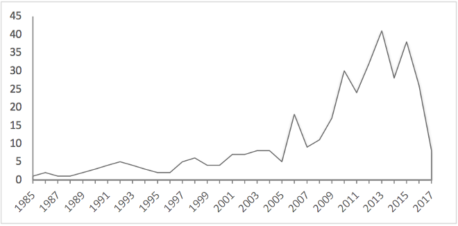
Although all states have enacted fair housing laws, only twenty-three states include a provision prohibiting sexual orientation discrimination in lending. Twenty of these states also prohibit gender identity discrimination. Table 1 lists the states that enacted fair housing laws prohibiting gender identity and/or sexual orientation discrimination, including the enactment and effective dates of the relevant statutes. Finally, two states, Arkansas and Tennessee, forbid their localities from adopting ordinances that would prohibit discrimination on a basis not recognized by the state.100 The result is that the same discriminatory behavior may be allowed in some states but not in others. Moreover, even in those states that do not prohibit discrimination in lending against members of the LGB community, discrimination may be prohibited in certain localities and counties. As Figure 1 below illustrates, the annual increase in the number of such political subdivisions sharply increased in 2010 and reached its highest point in 2013—the year following the enactment of the Equal Access Rule.

Table 1:  State Antidiscrimination Laws in Lending101

	Sexual Orientation		Gender Identity
State	Passed	Effective	Passed	Effective
CA	10/10/1999	10/10/1999*	09/06/2011	01/01/2012
CO	05/29/2008	05/29/2008	05/22/2014	08/06/2014
CT	05/01/1991	09/01/1993	07/01/2011	10/01/2011
DE	07/02/2009	07/02/2009	06/19/2013	06/19/2013
DC	12/13/1977	12/13/1977*	12/22/2005	03/08/2006
HI	07/11/2005	07/11/2005	07/11/2005	07/11/2005
IL	01/21/2005	01/01/2006	01/21/2005	01/01/2006
IA	05/05/2007	05/05/2007	05/05/2007	05/05/2007
ME	03/28/2012	09/01/2012	03/28/2012	09/01/2012
MD	05/15/2001	01/01/2001	05/15/2014	10/01/2014
MA	11/15/1989	11/15/1989	11/23/2011	07/01/2012
MN	04/02/1993	04/02/1993	04/02/1993	04/02/1993
NV	06/01/2011	06/01/2011	06/01/2011	06/01/2011
NJ	01/19/1992	01/19/1992	12/19/2006	06/17/2007
NM	04/08/2003	07/01/2003	04/08/2003	07/01/2003
OR	05/09/2007	01/01/2008	05/09/2007	01/01/2008
RI	05/22/1995	05/22/1995	07/13/2001	07/13/2001
UT	03/12/2015	05/12/2015	03/12/2015	05/12/2015
VT	04/23/1992	04/23/1992*	05/22/2007	07/01/2007
WA	01/31/2006	06/08/2006	01/31/2006	06/08/2006
NH	06/09/1997	01/01/1998	-	-
NY	12/17/2002	01/16/2003	-	-
WI	03/02/1981	03/02/1981*	-	-

Figure 1:  The Number of New Local-Level Protections against Sexual Orientation Discrimination in Jurisdictions without State-Level Protection102

D. An Under-studied Phenomenon

Of the very few studies that investigate sexual orientation discrimination, only two focus on the mortgage lending market.103 As we explain below, these studies were limited in nature. The first was a field experiment that was conducted in one state (Michigan), before the enactment of the Equal Access Rule, and had only 120 observations, of which only thirty-six focused on home financing.104 The second, written concurrently with this Article, was empirical in nature.105 This study treated all same-sex couples as one homogenous group, it focused on all mortgages (not just FHA loans), and it ignored the effect of state and local laws on acceptance rates. Importantly, due to their design, these studies could not provide—not even anecdotally—answers to the questions we investigate here. This Section begins with a short overview of the economics of discrimination. It then reviews the leading studies on sexual orientation discrimination and the shortcomings of their designs.

1. The economics of discrimination.

Discrimination in the home mortgage lending process is a topic that has received considerable attention both from academics and policymakers. In his seminal book, The Economics of Discrimination,106 Professor Gary Becker provided a basis for much of the theoretical work on discrimination.107 According to Becker, some individuals act as though they have a “taste,” or preference, for discrimination against a minority group.108 But discrimination comes at a cost: forgoing profitable transactions with members of the discriminated group.109

Theory predicts that in a competitive market, this cost will drive out taste-based discrimination.110 For example, an employer who prefers to hire only white employees forgoes the benefits that talented nonwhite employees may bring. Those employees may be hired by other firms and possibly at a lower than average salary. As a result, nondiscriminating firms may be able to offer better products or services at a lower price and consequently drive the discriminating firm out of the market.111 In the mortgage lending context, the cost of discriminating can also be prohibitive. Rejecting applicants with good credit because they belong to a certain group may result in fewer profits and a reduction in value. This is the case, for example, if the prejudicial lender reaches a point at which sales made to his preferred groups are exhausted. At that point, the prejudicial lender must either offer loans to all individuals or incur losses. Charging supracompetitive prices to members of a protected group (for example, reverse redlining112 ) is also infeasible if enough lenders are willing to offer credit.113 Markets, however, are not always competitive, and as a result, taste-based discrimination may persist.114

A different theory that explains why discrimination may persist in competitive markets, and can even be efficient, is statistical discrimination, meaning discrimination that arises out of a risk assessment based on characteristics commonly held by that group.115 Under this theory, firms do not discriminate because they have a taste for discrimination. Rather, in a world of imperfect information, these firms resort to group characteristics or stereotypes as proxies to evaluate outcome-relevant attributes of individuals. In other words, these firms make the inference that, because an individual belongs to a certain group, she possesses certain traits associated with that group. “In the classic textbook example, if employers believe (correctly) that workers belonging to a minority group perform, on average, worse than dominant group workers do, then the employers’ rational response is to treat [the two groups of workers] differently.”116 Another example is the use of a sex stereotype as a proxy in labor markets. Based on past experience, an employer may believe that, compared to men, women are more likely to leave their jobs during childbearing years. The behavior is rational and (likely) profit-maximizing even when the decisionmaker relies on proxies that are “over-broad generalizations and far from entirely accurate.”117

Redlining—the practice of denying services or raising prices to minority groups—can be the result of such statistical discrimination.118 Just like employers may rely on sex and race as proxies for performance,119 a lender may rely on similar proxies to estimate risk. As a result, what might appear to be systematic taste-based discrimination against a minority group may in fact simply be lenders avoiding loans in high-crime, low-income areas that happen to be heavily populated by the minority group. Economists refer to this form of discrimination as “statistical.” It is also referred to as rational discrimination,120 and some have argued that rational discrimination should be legally permitted.121

There are, of course, other theories of discrimination.122 Our goal here is not to review every possible theory. Rather, following the empirical literature, we focus on the taste-based and statistical discrimination theories.123 This focus allows us to reveal and propose new ways to deal with some of the flaws that plague previous studies. It also allows us to shed new light on and challenge their findings and conclusions. Finally, these two theories have another benefit: they interact differently with the Contact Hypothesis,124 a theory we test. Under this theory, discrimination may be the result of ignorance and, accordingly, can be reduced by contact with members of the minority group. If true, the empirical prediction is that areas with more intergroup contact experience less discrimination. The prediction holds when the discrimination is taste-based. By contrast, contact with minorities may reinforce statistical discrimination if it provides the decisionmaker with new proxies that will allow it to segment the market. For example, a lender who learns that members of a certain minority group suffer from a higher unemployment rate may refuse to sell them loans or require higher interest rates.125 If the lender learns through contact that certain groups are less likely to bargain, the lender may attempt to command higher prices. With these two theories in mind—taste-based and statistical discrimination—we now turn to the world of practice.

2. Two types of studies: the econometric approach and field experiments.

Attempts to empirically address taste-based and statistical discrimination have essentially taken two forms: (a) the econometric approach and (b) field studies. As we explain below, these studies suffer from a number of theoretical and methodological limitations. Understanding the criticism these studies faced and the methodologies they used not only motivates and informs our study but also allows us to extend the literature on discrimination in mortgage lending to discrimination based on sexual orientation.

a)  The econometric approach. The first approach is to maintain data at the individual level and assess the likelihood of loan acceptance. This is an attractive approach because lenders typically have guidelines and algorithms that drive the loan acceptance process. In a leading study, researchers were able to obtain all the data associated with whether a loan should have been accepted or denied.126 They were thus able to control for every factor that, according to the banks, was a relevant consideration. The study concluded that an application from a black or Hispanic individual was 8.2 percentage points less likely to be approved than an application filed by a white individual with similar bank-relevant characteristics.127 Follow-up studies questioned the sensitivity of this result and argued that, if anything, it applies only to applications right on the fringe of acceptance.128 Others argued that the single most important factor to a loan application—risk of loan default—is not adequately considered.129

The criticism that received possibly the most attention was that this type of modeling did not address the source of the discrimination, such as whether it was the result of taste-based or statistical discrimination.130 That is, was the observed discrimination evidence of bigotry? Or was race just a proxy for some other neighborhood characteristic associated with the typical black application that lenders might rationally want to avoid? Later studies attempted to answer the motivation question by aggregating the data away from the individual level to the neighborhood level. These studies found much weaker evidence of racial (taste-based) redlining.

As we discuss below,131 we are able to address each of the concerns brought up by the racial redlining literature—specifically that traditional techniques fail to disentangle race effects from neighborhood effects—in a number of ways available to us, thanks to the thoroughness of the HMDA data.132 By doing so, our study is not only the first to use regression-based analysis to study sexual orientation discrimination, but it also invites and sets the ground for future research.

b)  Field experiments. With very limited ability to obtain data on the individual level, “[m]uch of the research into housing discrimination, including HUD’s [Housing Discrimination Studies],” had to resort to “paired testing.”133 Under this methodology, “two testers assume the role of applicants with equivalent social and economic characteristics who differ only in terms of the characteristic being tested for discrimination, such as race, disability status, or marital status.”134

While most studies focus on racial discrimination in mortgage lending,135 only a few attempted to investigate sexual orientation discrimination. The first field experiment was conducted in Sweden in 2009 and found evidence of discrimination against same-sex couples.136 The authors sent out two fictitious applications for rental housing via the internet. One application was sent by a couple with a traditionally male and female name. The other application was sent by two distinctively male names, suggesting a gay couple. Each pair also presented itself as a “couple” to explicitly signal their sexual orientation. The authors then measured the rate at which each fictitious couple was called back. They found that, compared to the heterosexual couple, the homosexual couple was 14 percentage points less likely to receive a callback.137 A follow-up study carried out in much the same manner—email correspondence studies—found similar results in the Vancouver, Canada rental market.138

These two studies established some initial evidence of the possibility of discrimination based on sexual orientation, but they have their limitations. Because each study focuses on a specific area and addresses only rentals, we hesitate to draw too much of a conclusion about how these results might translate to mortgage approval rates. This is especially so because antidiscrimination laws differ from one country to another, as do social norms.

A broader concern is whether correspondence studies, which rely on response rates to email inquiries, can serve as a proper measure of discrimination. To begin with, such studies struggle to distinguish between taste-based and statistical discrimination because the underlying motivation for the housing denial is not known to the researcher and because the audit nature of these studies usually prohibits the use of neighborhood fixed effects. The distinction is critical, as different forms of discrimination call for different remedies and measures. Moreover, it is also unclear if the response rate can serve as a proxy for discrimination at all. The Swedish and Canadian studies exemplify the problem with the methodology. In both, a nonresponse was considered a negative outcome and a sign of discrimination.139 By contrast, all responses were considered nondiscriminatory outcomes even though there are many ways bigoted landlords can mask discrimination through a response. Examples are email replies that raise difficulties of actually seeing the apartment140 and responses that redirect the applicant to a different property owner—both of which happened in the Vancouver study.141 It is also likely that some prejudicial landlords provide untruthful responses regarding occupancy. These responses might be strong evidence of actual discrimination, but they were considered a nondiscriminatory outcome.

Another major challenge is whether the results, even if taken as valid, can be generalized. How much can a study in Sweden or Vancouver tell us about housing discrimination generally in the United States? In an effort to answer the question, HUD commissioned a similar email correspondence study.142 Touted as the “first large-scale [ ] study to assess housing discrimination against same-sex couples”143 on a “national scale,”144 the 2011 study conducted 6,833 paired email-correspondence tests across fifty randomly selected markets. The study found that, compared to heterosexual couples, same-sex couples—both male and female—received significantly fewer responses as compared to heterosexual couples.145 There was also some evidence that jurisdictions with state-level prohibitions against sexual orientation discrimination exhibited slightly more adverse treatment against same-sex couples compared with states without such prohibitions.146

The recent HUD study represents a new and improved generation of field experiments. Together with a recent study conducted in the automobile industry, it indicates that sexual orientation discrimination permeates many markets.147 But what the HUD and other studies did not and could not test is how sex and race interact. The automobile study included only white male testers, and in the HUD study, “the only difference between the two e-mails was whether the couple was same sex or heterosexual.”148

3. Sexual orientation in mortgage lending.

To date, only two studies have addressed sexual orientation discrimination in mortgage lending. The first study (Michigan Study) was conducted in 2007 by four of Michigan’s Fair Housing Centers and included 120 pair-tests.149 Each test included two pairs: one posing as a heterosexual couple and the other posing as a same-sex couple with superior credentials (“higher income, larger down payment, and better credit”).150 The study found disparate treatment in 32 (27 percent) of the 120 tests and concluded that discrimination against same-sex couples is widespread.151 The Michigan Study’s conclusion, however, suffers from a number of limitations. To begin with, the study focused on only one state: Michigan.152 The sample size was also small: a total of 120 paired tests.153 Third, the study focused on three markets, of which only 36 (or 30 percent) of the 120 tests were dedicated to discrimination in “home financing.”154 Moreover, home financing exhibited the least amount of discrimination: 20 percent compared to rental (33 percent) and homes sales (25 percent).155 Fourth, the study was conducted in 2007, five years before the enactment of the Equal Access Rule. At that time, discrimination on the basis of sexual orientation was allowed with respect to all types of mortgages, including FHA loans. Therefore, the study could not estimate the effectiveness of the Equal Access Rule.

The second study, conducted concurrently with ours, made a number of important findings.156 First, based on a national sample of 20 percent of HMDA data from 1990 to 2015, it found that, “compared to otherwise similar loan applicants,” the gross approval rate for same-sex couples is 3 percent lower.157 Merging the HMDA sample with Fannie Mae Performance Data revealed that same-sex couples whose applications were accepted were charged higher interests expenses at a magnitude of 0.02 to 0.2 percent.158 At the same time, the authors found no evidence that same-sex couples had a higher default risk.159 Professors Lei Gao and Hua Sun’s study makes an important contribution. But it is different from our study in a number of important respects, which do not allow it to answer the questions we investigate here. First, Gao and Sun’s study ignores the legal landscape and assumes that sexual orientation discrimination is not prohibited. Specifically, it ignores the fact that twenty-three states now prohibit sexual orientation discrimination in mortgage lending and that, even within states that do not prohibit the practice, some localities do. As a result, Gao and Sun did not and could not test the impact of state and local rules on acceptance rates. Gao and Sun’s study also does not separately measure discrimination by mortgage type. This could be potentially important, as FHA mortgages are subject to the Equal Access Rule while non-FHA mortgages are not.

Importantly, both studies were designed to test only one variable: sexual orientation discrimination. For this reason, these studies treated all same-sex couples, regardless of their sex (male/female) or race (black/white), as one homogeneous group.160 This design did not allow the authors to test how the interaction between sex and race influences the discriminatory practices identified.161 Nor could the studies identify the effect of local ordinances162 or determine whether and how “differences between the ways lesbians and gay men are treated” impacted the findings.163 Sun and Gao’s failure to distinguish between same-sex male couples and same-sex female couples may also explain the low level of discrimination found in their study—only 3 percent in the HMDA data.164 Our study suggests that same-sex female couples are treated at least as favorably (and in some cases more favorably) as heterosexual couples, which implies that the actual rate of sexual orientation discrimination against same-sex male couples is in fact higher.165

II. The Design, Data, and Findings

A. The Design

Our study is the first attempt to fill the gap and shed light on the very issues that the Michigan Study identified as important but left unanswered. As this Part explains, unlike the field experiments, we study sexual orientation discrimination in all states, using a large number of observations (over five million) and focusing solely on mortgage lending. Importantly, our study is the first to try to investigate how race and sex impact discrimination against same-sex applicants. Our data suggests that race is a critical factor, that lesbians and gay men are treated differently, and that state laws may have a real effect on discrimination against the LGB community.

Our study builds on the prior literature in a variety of ways. As Part II.B explains, based on the critiques of the use of individual-level data, we construct a model that remedies some of the problems identified in prior studies. Our model allows us to look at the individual effects of potential mortgage discrimination. It also takes into account the fact that different minority groups may self-select into neighborhoods and into mortgage applications that have a higher risk of default.

1. Risk considerations.

We take a number of steps to ensure we do not mistake legitimate risk considerations (including proxies that lenders may use to assess the risk of default, such as income or geographic effects) for discrimination. First, and exactly because of the concern that different applicants may carry different levels of risk, we focused only on FHA loans. Applicants for these loans must meet certain predetermined criteria.166 Importantly, for applicants who met the criteria, income and credit scores are less important. In the eyes of the lender, these FHA loans carry the same level of risk because each loan is insured by the federal government.167 This is not to say that FHA loans are risk-free. A high delinquency rate168 can translate into high servicing costs,169 costly regulatory review,170 and sanctions.171 It may also trigger indemnification requirements172 and can result in severe judgments173 and reputational harm.174 However, there is nothing to suggest that lenders believe that same-sex borrowers are more likely to default than other borrowers.175

Second, as we explain in the methodology section, while HMDA data is limited, we do have and control for the applicant’s income. That is, in addition to other controls, we compare loans of applicants with the same level of income.

Finally, we recognize that the neighborhood of the home may actually just be a proxy for bad credit (that is, bad economic neighborhoods generally attract applicants with bad credit). To control for a “neighborhood effect,” we include county-by-bank fixed effects, which controls for any differences across neighborhoods and banks. We are looking at how different compositions of race and gender affect loan acceptance within the same neighborhood by the same bank.176 Moreover, while we do not have the credit score of the applicant, we do know if the loan got denied because of a poor credit score. Thus, while we do not know the intimate details of an applicant’s credit history, we do know and control for those applicants with bad enough credit to disqualify them for an FHA loan. As we explain further below, our empirical design allows us to compare loans of similarly situated applicants (same applicant income, same loan amount, same loan purpose, same risk to the lender, etc.). This design—comparing loan acceptance rates within the same county by the same banks with multiple controls—has an important benefit. It offsets the concern that what we measure is actually just a proxy for some other neighborhood-level characteristic.

2. The proportion of same-sex gay co-applicants in the data.

Our design is still disadvantaged by a key element of sexual orientation discrimination. Other types of discrimination (for example, racial or gender) are typically based on characteristics that are easily observed by both the researcher and the lender. By contrast, sexual orientation is not a salient characteristic that the lender, much less the researcher, can necessarily observe. As a result, we do not and cannot directly observe applicants’ sexual orientation. While initially this may seem like a fatal flaw in our analysis, it is important to remember that the loan officer also does not directly observe sexual orientation. The loan officer can only infer sexual orientation based on observed characteristics (such as the applicant’s style of dress, behavior, etc.) and the perceived relationship between the applicant and co-applicant. While we do not (and cannot) observe sexual orientation, we do observe one important characteristic: whether the applicant is accompanied by a same-sex co-applicant. This is an important characteristic that loan officers observe.

We recognize that this is not a perfect proxy for the applicant’s actual sexual orientation. Indeed, co-applicants can be family members (for example, father and son) or friends, to give a few examples. However, there is strong theoretical and empirical evidence that our estimates do actually measure sexual orientation–based discrimination despite our inability to directly distinguish between same-sex homosexual co-applicants and same-sex heterosexual co-applicants.

a) Theoretical explanations. First, it is important to remember that the applicant’s true sexual orientation is irrelevant. Discrimination is not based on the actual sexual orientation of the applicant but rather on the applicant’s perceived sexual orientation. Discrimination is the result of what the loan officer believes to be true. By using same-sex co-applicants as a proxy for perceived sexual orientation, we are not only following in the footsteps of other researchers;177 we are also following the legal test established in Price Waterhouse. This test focuses on the plaintiff’s “appearance,” “behavior,” and “mannerisms,” as they were perceived by the loan officer.178

Moreover, our findings, if anything, are a conservative measure of the level of discrimination. The fact that we cannot distinguish between (a) same-sex heterosexual co-applicants and (b) same-sex gay co-applicants actually makes our results stronger. In other words, we show that, if the data includes not just gay co-applicants but also heterosexual co-applicants, then the true level of discrimination is actually higher than we report.

The reason is related to the first point: the loan officer cannot observe the co-applicants’ true sexual orientation. In some cases, the loan officer may have information that we cannot observe: for example, whether the same sex co-applicants are a father and son. In other cases, the loan officer may believe that the same sex co-applicants are a gay couple even if they are not. The concern, therefore, is that there are essentially two types of same-sex applications: (a) those applications in which the co-applicants are clearly related, such as a father/son pairing (Group 1), and are therefore not (or less likely to be) perceived179 as gay individuals, and (b) the rest of the same-sex applications, in which the relationship between the applicant and co-applicant is ambiguous to the lender (Group 2). As researchers, we cannot distinguish between Group 1 and Group 2. But if (i) the loan officer has a taste for discrimination and has additional information on the nature of the relationship either through last name or physical appearance (for example, Group 1 looks like a father and son versus Group 2, in which it is unclear), and (ii) the loan officer actually discriminates only against Group 2, then all that does is understate the magnitude of the effect of discrimination. In other words, the inability to distinguish between the two groups, if anything, biases our results toward zero.

To illustrate this point, consider the following example. Suppose the bigoted loan officer does not discriminate against Group 1 members because he has knowledge that is not observable to us as researchers. In such a case, members of Group 1 are 0 percent more/less likely to have the loan approved (that is, they will be treated the same as the white heterosexual benchmark). Now, because the loan officer is bigoted and does like to discriminate against Group 2 members (perceived gay co-applicants), those loans are, say, 12 percent less likely to get accepted. The “true” level of discrimination is 12 percent. However, in our analysis, we necessarily are forced to clump Group 1 and Group 2 loans together. Our resulting estimates average the effect of Group 1 and Group 2, which in this hypothetical would result in an overall effect of loans 6 percent ([0+12]/2) less likely to be approved. Thus, if anything, this ambiguity only understates the level of discrimination (“true” level of 12 percent compared to the estimated effect of 6 percent) but does not invalidate our estimates.

b) Empirical evidence. We further this claim empirically in three ways. First, we track the rate of same-sex loan applications in states and local jurisdictions that passed laws prohibiting discrimination on the basis of sexual orientation.

Figure 2:  Change in Same-Sex Loan Applications before and after the Passage of Antidiscrimination Laws

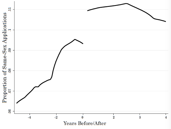
Figure 2 above tracks the proportion of same-sex loan applications over time, centered on the year the law passed (because not all laws are passed in the same year). The horizontal axis measures time in years before and after the law is passed, and the vertical axis measures the proportion of same-sex loans. As Figure 2 demonstrates, there is a marked increase in same-sex loans after the law passes that persists through the end of our data range. Under the assumption that the Group 1 (perceived heterosexual co-applicants, such as parent-child) same-sex loans will not be affected by changes in anti–sexual orientation discrimination laws, Figure 2 suggests that laws are specifically opening the door for more Group 2 (perceived gay co-applicants) loans.

Figure 2 is also consistent with previous research showing that same-sex loan applications increased after the decision in Obergefell v Hodges.180 This study, conducted by HUD in 2016, exploited the “variation across states prior to the Supreme Court decision to investigate the effect of marriage laws on demand for mortgage credit.”181 By using the same methodology that we do—looking at the reported sex of co-applicants—it concluded that states that passed same-sex marriage laws “experienced [an] 8 to 13 percent increase in same-sex mortgage applications.”182

Figure 3:  The Relationship between the Size of the LGBT Community and the Proportion of Same-Sex Loans by State183

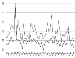
Second, Figure 3 shows that the number of loan applications with two co-applicants of the same sex correlates to the size of the LGBT community. This suggests that many of the same-sex loan applications in our dataset were submitted by gay or lesbian couples rather than other same-sex co-applicants, such as roommates or relatives of the same sex. In Figure 3, we compare the proportion of same-sex loans per state—the top line—to the actual proportion of individuals in the state that consider themselves part of the LGBT community—the lower line.184 Both lines trend together, with a correlation coefficient of 0.71, suggesting a strong and robust correlation. Essentially, in states with a larger LGBT community, more same-sex applications are filed. Figure 3 therefore suggests that most of the same-sex applications we measure are, in fact, home loan applications filed by gay co-applicants. Part II.C reports the result of a third robustness test leading to the same conclusion.

B. The Model

1. The data and methodology.

Our study relies on three datasets. The first two are proprietary and include state- and local-level protection against antidiscrimination practices in mortgage lending.185 The third has publicly available data on home mortgages reported by financial institutions pursuant to the HMDA. We study every home loan application in the United States reported under the HMDA between the years 2010 and 2015—about five million observations.186 To keep the risk of the loan constant, we restrict the dataset to include only applications made for FHA loans in which the applicant has a co-applicant.187

Our outcome of interest is an indicator variable signifying whether or not the loan was accepted. The variable equals 1 if the loan was accepted and 0 if the loan was rejected.188 In addition to the gender and racial makeup of the applicant and co-applicant, we are able to control for a myriad of factors that influence the probability of whether a home loan is accepted. These include the applicant’s income, loan amount, property type,189 loan purpose,190 whether or not the home will be owner occupied, whether or not the applicant had been preapproved, the applicant’s ethnicity, and the reason for denial, if any. We include each of these variables in each model to account for any observable factor that may influence the bank’s decision to accept or deny the loan.

To account for any national, unobserved trends in the data, we also include in each model year-fixed effects. These dummy variables allow us to control for changes in home loan trends that are common across all loans in a given year.191

Additionally, we control for variation between different banks in the same county and different branches of the same bank in different counties. To see why, suppose that Bank I and Bank II are large national banks with branches in numerous counties in the United States. Bank I may have different lending practices than Bank II. Similarly, a branch of Bank I in one county may have different lending practices than a branch of Bank I in a different county. To control for these two forms of variation (interbank and intrabank), we create a dummy variable for each bank in each county. That is, we create a set of dummy variables for Bank I for each county in each state, and we do the same for all the other banks. These bank-by-county fixed effects absorb all crossbank and crosscounty differences. All the variation that remains is the differences in lending practices within banks in the same county. Put differently, including these fixed effects allows us to look at how the same bank in the same county treats different applications. These variables allow us to exploit the within-bank and within-county variation.192

Discrimination is a comparative term. Accordingly, our comparison group is the white male/white female pair—the most common combination in the dataset. Our independent variables are a set of all the remaining fifteen possible gender and race combinations between a primary applicant and a co-applicant. We thus have a separate dummy variable for each of the following combinations: (1) white male/black male, (2) white male/white male, (3) black male/black male, (4) black male/white male, (5) white female/black male, (6) white female/white male, (7) black female/black male, (8) black female/white male, (9) white female/black female, (10) white female/white female, (11) black female/black female, (12) black female/white female, (13) white male/black female, (14) black male/black female, (15) black male/white female.

Formally, Equation 1 estimates the following linear probability model:

Where Libcy represents whether or not loan application i was accepted at bank b in county c in year y. Xibcy is a matrix of covariates that influence the probability a home loan is accepted,193 τy is a set of time-fixed effects, ρbc is the set of bank-by-county fixed effects, and eibcy is the error term. The remaining fifteen variables measure the effect of each unique pair of race and gender combinations. Accordingly, the coefficient bk can be interpreted as the percentage point change in the probability of loan acceptance. The omitted group is a white male applicant with a white female co-applicant.

2. Model validity.

HMDA data is rich and provides the most complete coverage of the loan application process.194 Still, there are many concerns that need to be addressed.

a)  Linear probability modeling. A restricted dependent variable, such as a binary outcome of whether or not a loan was accepted, violates the assumptions of ordinary least squares estimation (OLS), in part because the dependent variable is not continuous but also because the standard errors are misestimated. Additionally, it is possible for a linear probability model (OLS applied to a binary outcome variable) to produce model estimates that yield a nonsensical predicted probability that is greater than one. Alternative estimation techniques such as logit and probit models correct for this by constraining the model to be bound between zero and one. These models, however, come with their own set of assumptions and perform equally as poorly, if not worse, than linear probability models.195

In the context of this Article, we are able to alleviate the typical concerns associated with linear probability modeling. First, we adjust for bias in the estimation of the standard errors by clustering the standard errors in each model at the state level. Second, in our dataset, 47 percent of the loans we analyze were accepted. Thus, the oft-voiced critique that linear probability models perform poorly when there are very few events (that is, no loans were accepted) or very few nonevents (in other words, almost all loans are accepted) is not an issue.196 Lastly, we are mostly interested in calculating marginal effects for each of the pair combinations and less concerned about making predictions or forecasts of the full model. Accordingly, the concern that a linear probability model could produce predictions of a probability greater (or less) than one is not an issue. We turn to review other potential pitfalls discussed in the home mortgage literature, which are not specific to Equation 1.

b)  Demographics as an endogenous instrument for economic conditions. Many early studies of home mortgage discrimination pointed to the possibility of race, or any other demographic, as nothing more than a proxy for another, unobserved variable.197 For instance, if blacks disproportionally apply for home loans in more economically disadvantaged neighborhoods, lenders may be more likely to deny the loan application. The reason is not due to racial discrimination but rather due to the perceived high risk of extending a loan to applicants residing in such neighborhoods. As we previously mention, economists often refer to this type of discrimination as statistical discrimination: discrimination that is based on a factor other than a demographic characteristic.

Our study finds more conclusive evidence that the motivation for discrimination is taste-based, or bigotry, than any previous econometric study. The reason is that, unlike with race, lenders are less likely to rely on perceived sexual orientation as a proxy for increased risk.198 Moreover, given the sheer magnitude of the dataset HMDA offers, we are able to control for lender-by-county fixed effects. That is, our analysis compares loan applications considered by the same lender from those who reside in the same county, which by definition has the same risk to the lender (they are all FHA loans).199 It is thus very likely that the reason for any disparate treatment was not based on factors relevant to risk assessment but on the applicants’ perceived sexual orientation.200

c)  Risks observed by the bank but not by the researcher. There is also some concern that there are factors that the lenders are able to observe and include in a risk assessment of the loan application that we, as researchers, are not able to observe in the data. The most glaring example is credit scores, which are probably the single strongest indicator of risk and are a factor observed by the lender.201 Despite its richness, HMDA does not include credit scores. However, as Part II.A.1 explains above, our research design allows us to address and mitigate this concern in a myriad of ways, one of which is by focusing solely on FHA loans.202 The unique feature of these loans is that they carry the same low level of risk to the lender. An applicant approved for an FHA loan pays an FHA insurance premium. In case of a default, the lender recoups the losses from the government.203 As a result, every FHA loan bears the same risk and expected return to the lender regardless of the demographic characteristics of the applicant. Accordingly, it is unlikely that disparate treatment in FHA loan denial can be traced to an unobserved (to the researcher) measure of risk.

C. Results

The results for our main analysis of Equation 1 can be seen in Table 2 and graphically in Figure 4.

Table 2:  Probability of Loan Acceptance by Race and Gender204

Applicant	Co-applicant	(1)	(2)
White Male	Black Male	-0.038** (0.017)	-0.043*** (0.014)
White Male	White Male	-0.021*** (0.005)	-0.025*** (0.003)
Black Male	Black Male	-0.087*** (0.008)	-0.075*** (0.009)
Black Male	White Male	-0.070*** (0.014)	-0.068*** (0.011)
White Female	Black Male	0.012*** (0.004)	0.040*** (0.005)
White Female	White Male	0.012*** (0.001)	0.037*** (0.003)
Black Female	Black Male	-0.038*** (0.004)	0.005 (0.003)
Black Female	White Male	-0.007 (0.008)	0.019*** (0.006)
White Female	Black Female	-0.028 (0.017)	0.014 (0.015)
White Female	White Female	-0.012*** (0.002)	0.027*** (0.006)
Black Female	Black Female	-0.062*** (0.006)	-0.011 (0.007)
Black Female	White Female	-0.043*** (0.015)	-0.006 (0.017)
White Male	Black Female	0.006* (0.003)	-0.002 (0.003)
Black Male	Black Female	-0.033*** (0.003)	-0.021*** (0.002)
Black Male	White Female	0.011*** (0.002)	0.005** (0.002)
	Controls Sample Size R Squared	5,864,086 0.32	X 5,864,086 0.42

In Table 2, Column (1) estimates Equation 1 with the inclusion of year and bank-by-county fixed effects, but with no other controls. Column (2) reports the results with the controls mentioned previously.205 In both models, the corrected standard errors clustered at the state level are in parentheses. Each coefficient can be interpreted as the percentage point increase (if positive) or decrease (if negative) in the likelihood of a loan to be accepted for each applicant/co-applicant pair relative to a white male/white female applicant pair. For instance, from Column (2) in Table 2, a pair consisting of a white male applicant and a black male co-applicant is 4.3 percentage points less likely to have a loan accepted as a white male/white female pair asking for the same loan amount with the same income from the same lender in the same county. This means that, if a white male/black male pair has a 45 percent chance of having a loan application accepted, we would expect a white male/white female pair to have a 49.3 percent chance of approval. This is so despite the fact that both pairs requested the same amount for the same purpose with the same income from the same lender in the same county and bear the same level of risk to the lender.

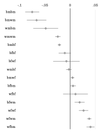
Figure 4:  Effect of Gender and Racial Composition on Co-applicant Loan Acceptance206

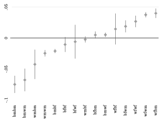
Figure 4 organizes the results in Table 2 from most negative to most positive and includes bands that represent 90 percent confidence intervals. To interpret Figure 4, focus first on the points at the center of the intervals. A point that lies below the zero line suggests the race/gender pairing is less likely to have a loan accepted, and a point above the line suggests the acceptance is more likely. Now focus on the intervals. If an interval intersects with the zero line on the horizontal axis, the estimated effect is not statistically significant at the 10 percent level.

To test once again whether the results are driven by same-sex gay co-applicants (rather than by same-sex heterosexual parent-child co-applicants),207 we remove from the dataset any applicant or co-applicant that reports more than one race. The rationale is that keeping only “single-race” applicants would (likely) exclude from the data parent-and-child co-applicants. The reason is that it is unlikely that a co-applicant who reports one race (for example, black) will be the parent of the applicant with only one different race (for example, white). We report the results of this regression graphically in Figure 5 below. Figure 5 shows that, when the sample is restricted to the types of same-sex loans that are more likely representative of actual gay couples (Group 2208 ), the results hold and in some cases are slightly stronger.

Figure 5:  Effect of Gender and Racial Composition on Application Success When the Loans Are More Likely to Be Submitted by Gay Couples

The empirical evidence suggests that a large portion of the same-sex loan applications are actually loans submitted by gay couples. Moreover, the differences between the results that Figures 4 and 5 report are also consistent with our theoretical prediction in Part II.A that our results are a conservative measure of discrimination and that the actual level of discrimination is higher than we observe.

1. National patterns in discrimination.

With this in mind, we turn to analyze the results. Figure 4 provides strong evidence of systemic and widespread discrimination against gay male couples. More specifically, Figure 4 shows that any application with a pair of males is statistically less likely to be approved relative to the same white heterosexual pair. Within the same-sex male pair groups, race plays a role. Although all same-sex male applications are less likely to be accepted, black-male pairs are the least likely to be approved (-7.5 percentage points), followed by the interracial pairs of black male/white male (-6.8), white male/black male (-4.3) and white male pair (-2.5). Interestingly, the exact same pattern holds for female pairs. From the least to most likely to be approved are black female pairs, followed by interracial black female/white female and white female/black female pairs, and white female pairs. In the case of same-sex pairs (that is, male/male and female/female pairs), the data reveals some evidence of a statistically significant “primary applicant” effect. The differences between interracial pairs, however, are statistically indistinguishable from one another.

Our results shed new light on earlier studies of discrimination. Previous research has suggested significant and persistent evidence of racial discrimination in mortgage lending. Recent estimates suggest that black pairs are 7 percentage points less likely to have a loan accepted.209 The evidence we present here suggests the possibility of a more nuanced story. While race seems to play an important role in the probability of getting a home loan, interracial applicants and even white male pair applicants are statistically less likely to get accepted. The fact that even white male pairs are less likely to get a loan in a similar fashion to other same-sex male pairs is important for at least two reasons. First, it is evidence of discrimination on the basis of sexual orientation that is consistent with the pair-studies literature. Second, the evidence of discrimination against white male pairs alleviates the concern that Figure 4 measures nothing more than racial discrimination. Finally, even after we control for the gender composition of the same-sex pair applicants, we do find that, compared to the white heterosexual baseline, a pair consisting of a black male and a black female is still statistically less likely to have a home loan application accepted. The effect, however, is about half as small as previous estimates.210

Another interesting finding in our results is the lack of symmetry of effect between perceived gay and perceived lesbian co-applicants. We find that every possible racial combination of male pairs is statistically disadvantaged when getting a loan application approved. By contrast, in every case, a female pair is either statistically indistinguishable from the baseline group or actually has a higher likelihood of getting the loan accepted. This result is actually consistent with much of the experimental literature on sexual orientation discrimination in housing211 and coincides well with the growing body of literature about the social acceptability of lesbian, but not gay male, relationships.212

It is important to remember that we do not observe the nature of the relationship between the co-applicants in the data.213 However, unlike other salient bases for discrimination (such as race), sexual orientation is much harder for the loan officer to observe. In many cases, the loan officer does not know with certainty either the orientation of the applicants or their relationship. In the absence of a clear signal, the discriminatory loan officer (either overtly or inadvertently) likely uses the gender and race of the co-applicants as a proxy for sexual orientation. We, in effect, use the same proxy in this study. The proxy is admittedly imperfect. Surely there are times that the bias, even an intentional one, would be the result of a mistake. For instance, the loan officer may mistakenly believe that a pair of heterosexual male applicants is involved in a homosexual relationship. These heterosexual applicants may thus receive the same discriminatory treatment as if they were gay. In our eyes (and in the eyes of the law), this does not mean the analysis is flawed. All it means is that discrimination is happening against gay applicants and applicants who are perceived to be gay. What could result, potentially, is actually “overdiscrimination”—that is, discrimination against the targeted group and, in addition, discrimination against others who are perceived as belonging to the targeted group.

2. Regional patterns in discrimination.

The results that Table 2 and Figure 4 report above compare loan applications to other loan applications from the same bank in the same county, in order to control for external variables, and then aggregate the results for the entire country by race and gender pairings. There may be reason, however, to believe that different regions in the United States or different types of banks discriminate differently. To control for this, we first divide the data into four census regions, re-estimate Equation 1, and replicate Table 2 and Figure 4. Instead of looking at the effect of a gender and race applicant makeup of, say, black male/black male, we divide that single dummy variable into four variables that signify whether the loan was filed by (a) a pair of black males in the West, (b) a pair of black males in the South, (c) a pair of black males in the Midwest, or (d) a pair of black males in the Northeast.214 We do this for each of our fifteen gender and race indicator variables of interest and include them all in the regression. What results is an estimate of the probability of loan acceptance for each group by region. Those results are summarized in Table 3 and Figure 6 below.

Table 3:  Probability of Loan Acceptance by Race, Gender, and Region215

Applicant	Co-applicant	Northeast	Midwest	South	West
White Male	Black Male	-0.122*** (0.030)	-0.018 (0.035)	-0.027* (0.016)	-0.015 (0.027)
White Male	White Male	-0.023*** (0.005)	-0.019*** (0.005)	-0.020*** (0.004)	-0.033*** (0.005)
Black Male	Black Male	-0.076*** (0.006)	-0.086*** (0.015)	-0.076*** (0.013)	-0.052*** (0.007)
Black Male	White Male	-0.078*** (0.010)	-0.072** (0.031)	-0.061*** (0.020)	-0.065** (0.032)
White Female	Black Male	0.033** (0.012)	0.035*** (0.010)	0.042*** (0.007)	0.046*** (0.006)
White Female	White Male	0.037*** (0.003)	0.037*** (0.003)	0.039*** (0.003)	0.036*** (0.002)
Black Female	Black Male	0.006* (0.003)	-0.001 (0.004)	0.007 (0.004)	0.005 (0.004)
Black Female	White Male	0.027*** (0.004)	0.041*** (0.013)	0.006 (0.009)	0.021* (0.012)
White Female	Black Female	-0.008 (0.024)	0.031 (0.046)	0.021 (0.021)	0.016 (0.027)
White Female	White Female	0.026*** (0.005)	0.026*** (0.007)	0.028*** (0.005)	0.026*** (0.008)
Black Female	Black Female	-0.003 (0.007)	-0.027*** (0.010)	-0.004 (0.008)	-0.040*** (0.008)
Black Female	White Female	0.033 (0.021)	-0.032 (0.022)	-0.007 (0.010)	-0.017 (0.044)
White Male	Black Female	0.009 (0.012)	-0.009 (0.007)	-0.005 (0.004)	-0.001 (0.004)
Black Male	Black Female	-0.019*** (0.004)	-0.029*** (0.005)	-0.019*** (0.003)	-0.021*** (0.002)
Black Male	White Female	0.017*** (0.002)	0.002 (0.004)	0.005 (0.004)	0.001 (0.003)
	Sample Size R Squared	5,864,086 0.42

Table 3 and Figure 6 indicate that all regions in the United States exhibit the same pattern of discrimination we observe on the national level. In each region, all four groups (male, female, black, and white applicants) are discriminated against based on perceived sexual orientation. In other words, all applications filed by same-sex pairs are less likely to be accepted compared to the white heterosexual pair. In certain circumstances, the negative effect is statistically insignificant, but it is still negative. For instance, in the Midwest, an application filed by an interracial same-sex pair consisting of a white male and black male pair is statistically indistinguishable from zero. By contrast, an application filed by other same-sex male pairs is statistically less likely to get accepted by the same bank in the same county as the white heterosexual pair application. That same group of applicants—white male/black male—is also statistically insignificant in the West, but again, each of the other three highlighted same-sex groups are still statistically worse off. Interestingly, the data suggests that this interracial pair is discriminated against most in the Northeast. In that region, applications from white male/black male pairs are 12.2 percentage points less likely to be approved. The result is not only the worst in magnitude but also the most statistically significant (at the 99 percent level).

Figure 6:  Effect of Gender and Racial Composition on Co-applicant Loan Acceptance by Region216

Based on the results in Figure 6, there is no evidence that any single region in the United States is driving the results. There may have been a temptation to blame certain regions of the United States for the discrimination that seems to be occurring. However, the data suggests that discrimination based on (perceived) sexual orientation is widespread and not isolated to any specific geographic region. Put differently, no region is insulated from those discriminatory behaviors.217

To explore this point further, we repeat the regional analysis above, but instead of splitting the data by region, we split it by political party lines. To do so, we sort each state into one of three

categories: states commonly considered “blue” states that basically always vote Democrat in a presidential election,218 “red” states that basically always vote Republican in a presidential election,219 or “swing” states220 that could go either way. The results for this regression are summarized in Table 4 and Figure 7.

Table 4:  Probability of Loan Acceptance by Political Party Lines221

Applicant	Co-applicant	Democrat	Republican	Swing
White Male	Black Male	-0.068** (0.026)	-0.040* (0.021)	-0.008 (0.021)
White Male	White Male	-0.033*** (0.005)	-0.017*** (0.005)	-0.021*** (0.004)
Black Male	Black Male	-0.068*** (0.009)	-0.071*** (0.010)	-0.088*** (0.015)
Black Male	White Male	-0.087*** (0.019)	-0.044** (0.020)	-0.062*** (0.017)
White Female	Black Male	0.034*** (0.006)	0.042*** (0.005)	0.044*** (0.010)
White Female	White Male	0.036*** (0.003)	0.039*** (0.003)	0.038*** (0.003)
Black Female	Black Male	0.007* (0.004)	0.009** (0.003)	-0.002 (0.005)
Black Female	White Male	0.023*** (0.006)	0.011 (0.011)	0.022 (0.014)
White Female	Black Female	0.005 (0.016)	0.020 (0.033)	0.024 (0.024)
White Female	White Female	0.022*** (0.005)	0.031*** (0.005)	0.028*** (0.005)
Black Female	Black Female	-0.008 (0.010)	-0.006 (0.008)	-0.021** (0.010)
Black Female	White Female	-0.008 (0.029)	-0.015 (0.016)	0.005 (0.018)
White Male	Black Female	0.005 (0.006)	-0.006 (0.005)	-0.009 (0.005)
Black Male	Black Female	-0.020*** (0.002)	-0.016*** (0.002)	-0.030*** (0.003)
Black Male	White Female	0.004 (0.003)	0.008* (0.004)	0.003 (0.002)
	Sample Size R Squared	5,864,086 0.42

To compare the patterns of discrimination based on political party lines to those observed in the national pattern, Figure 7 includes the graph from Figure 4. Similar to the analysis by region, we see no obvious pattern that follows party lines. While there are some differences for specific groups across party lines, most of those differences are small and statistically insignificant. Thus, while the magnitude of the effect varies slightly, the application of a pair consisting of two black males is no better positioned to be accepted in, for example, Utah than in Oregon or Wisconsin (all else equal). One interesting exception is that Democratic states are the least tolerant to the two groups of interracial male pairs. The results are not only substantially stronger in magnitude—in the case of the black/white male pair, the chance to be approved in a Democratic state is about half compared to that in Republican states—but they are also most statically significant. More broadly, Figure 7 demonstrates that these lending patterns cannot be attributed simply to the mindset of a specific region or a certain political philosophy. These patterns of discrimination are widespread and can be observed in virtually every geopolitical segment of the United States.

Figure 7:  Effect of Gender and Racial Composition on Co-applicant Loan Acceptance by Political Party Lines222

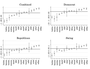
One last potential source of variation that may be driving the results is not necessarily the makeup of the community but rather the lenders themselves. Though unlikely, given the within bank-county analysis we conduct in this study, there may be something about the way large versus medium or smaller banks operate that may inform the results we present here. For example, one could argue that larger banks are less likely to discriminate because, among other possible reasons, they may have better procedures or higher exposure. To test this, we split out the data by the ten largest banks in terms of loan applications received. These banks make up about 40 percent of the loan applications in our database. We then compare the “Top Ten” banks to all banks in the smallest 25 percent by loan applications handled and all other medium banks in between.223 The results, which Table 5 and Figure 8 present, suggest a very similar pattern. Large, medium, and smaller banks act very much in the same way.

Table 5:  Probability of Loan Acceptance by Race and Gender and Bank Size224

Applicant	Co-applicant	Ten Largest Banks	Medium Banks	Smallest Banks
White Male	Black Male	-0.019 (0.022)	-0.056** (0.025)	-0.060** (0.026)
White Male	White Male	-0.026*** (0.004)	-0.023*** (0.005)	-0.026*** (0.004)
Black Male	Black Male	-0.040*** (0.009)	-0.098*** (0.013)	-0.102*** (0.013)
Black Male	White Male	-0.056*** (0.016)	-0.062*** (0.020)	-0.105*** (0.026)
White Female	Black Male	0.031*** (0.006)	0.042*** (0.007)	0.057*** (0.011)
White Female	White Male	0.036*** (0.002)	0.039*** (0.003)	0.039*** (0.003)
Black Female	Black Male	0.025*** (0.004)	-0.010** (0.005)	-0.013** (0.005)
Black Female	White Male	0.019** (0.009)	0.020** (0.009)	0.014 (0.013)
White Female	Black Female	0.010 (0.022)	0.020 (0.021)	0.009 (0.034)
White Female	White Female	0.024*** (0.005)	0.030*** (0.007)	0.025*** (0.006)
Black Female	Black Female	0.017** (0.007)	-0.031*** (0.010)	-0.026** (0.012)
Black Female	White Female	-0.032 (0.022)	0.005 (0.022)	0.018 (0.025)
White Male	Black Female	-0.014** (0.006)	0.002 (0.006)	0.013* (0.007)
Black Male	Black Female	-0.003 (0.004)	-0.035*** (0.002)	-0.033*** (0.004)
Black Male	White Female	-0.003 (0.005)	0.011*** (0.004)	0.008* (0.004)
	Sample Size R Squared	5,864,086 0.42

Figure 8:  Effect of Gender and Racial Composition on Co-applicant Loan Acceptance by Bank Size225

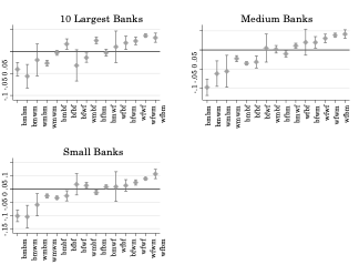
It is important to note, however, that among the largest banks, the magnitudes of the effects of race and sexual orientation are smaller in ways that are, at times, meaningful. For instance, an application filed by a pair consisting of two black male co-applicants at one of the ten largest banks is only 4 percentage points less likely to get accepted than that of a white heterosexual pair. The same pair is 9 percentage points less likely to get accepted at all other banks. Also, the effect for applications filed by interracial pairs consisting of white male and black male co-applicants is much smaller and statistically insignificant for big banks.

3. Remedies for reversing trends of systematic and widespread bias.

The evidence we present here suggests a systematic and widespread bias against FHA loan applications filed by any male pair, regardless of race. It may be the case, though, that the reason for these discriminatory patterns is more nuanced. For instance, it could be that the results are not an artifact of regional differences in attitudes or political opinions but the lack of contact with the affected group. Assuming this is true, what can be done to remedy the situation?

a)  The “Contact Hypothesis.” To understand the Contact Hypothesis, suppose the average loan officer identifies as straight and has well-established biases against the LGB community—specifically, biases against gay men. Research shows that efforts to reduce such intergroup bias in a meaningful and enduring way demand thorough and intense intervention over a long period.226 One type of intervention that has had some reported effect in reducing intergroup bias is sustained contact with individuals of the affected group.227 The idea behind the prevailing (yet debated) Contact Hypothesis is that, under certain conditions, intergroup bias would decrease as individual contact between different groups’ members increases.228

Could it be that our results are being driven by a lack of sustained contact with the affected groups? We test this by comparing loan acceptance rates between urban and rural environments. Under the Contact Hypothesis, one would expect to observe less discrimination in urban environments. Based simply on sheer population numbers, it is likely that the average loan officer operating in an urban area has a higher chance of sustained contact with gay men. We loosely define an environment as urban if its population density is above average and as rural if its population density is below average.229 Table 6 and Figure 9 below report the results for each of the gender and race pair variations in these environments.

Table 6:  Probability of Loan Acceptance by Race, Gender, and Population Density230

Applicant	Co-applicant	Rural	Urban
White Male	Black Male	-0.039** (0.015)	-0.048** (0.022)
White Male	White Male	-0.025*** (0.003)	-0.025*** (0.003)
Black Male	Black Male	-0.082*** (0.010)	-0.067*** (0.009)
Black Male	White Male	-0.054*** (0.018)	-0.082*** (0.015)
White Female	Black Male	0.039*** (0.007)	0.041*** (0.006)
White Female	White Male	0.035*** (0.003)	0.040*** (0.003)
Black Female	Black Male	0.005 (0.003)	0.005 (0.005)
Black Female	White Male	0.020*** (0.007)	0.017* (0.009)
White Female	Black Female	0.004 (0.018)	0.026 (0.018)
White Female	White Female	0.025*** (0.005)	0.029*** (0.006)
Black Female	Black Female	-0.011* (0.007)	-0.010 (0.010)
Black Female	White Female	0.010 (0.020)	-0.023 (0.022)
White Male	Black Female	-0.013*** (0.004)	0.009* (0.004)
Black Male	Black Female	-0.026*** (0.002)	-0.017*** (0.002)
Black Male	White Female	0.000 (0.004)	0.010*** (0.003)
	Sample Size R Squared	5,864,086 0.42

Figure 9: Effect of Gender and Racial Composition on Co-applicant Loan Acceptance by Population Density231

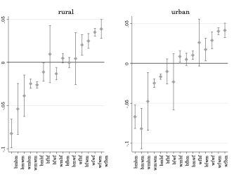
We find the same pattern of systemic discrimination with virtually no evidence of any difference in loan application acceptance between rural and urban environments. While the point estimates in Figure 9’s two graphs vary slightly, the differences are not significant, and each of the four disadvantaged male pair groups232 is still less likely to get a loan approved in a statistically significant way. Thus, if comparing rural to urban settings is a reasonable proxy for association with gay men, it appears that contact alone may not reduce intergroup bias.

b)  State and local laws. As we explain earlier, discrimination based on sexual orientation is not prohibited under federal law.233 In light of federal inaction, twenty-three states and over four hundred localities passed laws expressly prohibiting discrimination based on sexual orientation in lending.234 These local laws may influence lenders’ behaviors. The reason could be intrinsic. Expressive law theorists, for example, argue that “the mere existence of [a] law helps to shape and define [people’s] world views” and increase compliance.235 Or the reason may be extrinsic. For example, it could be that local laws result in increased compliance due to enforcement efforts or fear thereof. Alternatively, it could be that jurisdictions that adopt local antidiscrimination laws do so because they are already more accepting of gay applicants.

Whatever the reason may be, it is clear that the minority of states and localities that adopted these laws were not selected randomly to do so. This is important because, hypothetically, the best way to measure the efficacy of a law, policy, or any type of policy intervention would have been to randomly assign the law to half the states and localities and keep the remaining half as a control group. In this hypothetical, states and localities would have no control over whether they got the law; thus, any difference in the underlying characteristics between the states and localities would be random. The reality, however, is that antidiscrimination laws are not randomly assigned to state and local jurisdictions. Similarly, states and localities that declined to adopt such protections did not randomly choose to refrain from doing so. This calls into question their validity as the comparison group and could bias the results.236 This bias would manifest if we simply compared states with antidiscrimination laws to states without such laws.237 To alleviate this potential source of statistical bias, we focus only on states and localities that changed their laws within the time window of our dataset, 2010 to 2015. This allows us to compare the same local jurisdiction to itself before and after it passed the law. Only three states—Maine, Nevada, and Utah—and 174 local municipalities changed their laws during this window. These states and localities processed almost a quarter million loan applications from 2010 to 2015.

To analyze the effectiveness of local laws, we employ a difference-in-differences regression technique. This technique, common in policy analysis,238 is a method that helps alleviate the lack of an appropriate baseline group by focusing on two baselines. The method works as follows: First, we focus on jurisdictions that adopted local laws. Each such jurisdiction is compared to itself. Specifically, we calculate the acceptance rate in that jurisdiction before the local law was passed and compare it to the rate after it was passed. This generates the first difference. For example, Nevada passed a law prohibiting sexual orientation discrimination in 2011, and it went into effect that same year. Therefore, the first step is comparing Nevada to itself. To calculate the first difference, the regression calculates the difference in loan acceptance rates for Nevada before and after the effective date. That is, we compare the acceptance rate from 2011 to 2015 to the rate in 2010.

This first difference, however, is not enough. It could be that, during the year the law changed, other factors that are not unique to Nevada influenced the results. For example, it could be that a regional crisis influenced the acceptance rate in Nevada. To account for this, the regression calculates the change in acceptance rates between 2011 and 2015 compared to those in 2010 in jurisdictions that did not adopt a local rule. This is the second difference. It then compares the first difference to the second one.239 The idea is that, while the assignment of the law is still not random, using this technique filters out any factor relevant to the outcome of interest. Thus, all that remains is the effect of the law and random noise not relevant to the law or the outcome.240

The results of the difference-in-differences estimates of the effect of state and local antidiscrimination laws are presented in Table 7 and Figure 10.

Table 7:  Probability of Loan Acceptance by Race and Gender in States with Changes to City or State Law241

Applicant	Co-applicant	State Law
White Male	Black Male	-0.086 (0.074)
White Male	White Male	-0.001 (0.008)
Black Male	Black Male	-0.031** (0.015)
Black Male	White Male	-0.014 (0.057)
White Female	Black Male	0.012 (0.015)
White Female	White Male	0.004 (0.003)
Black Female	Black Male	-0.024*** (0.006)
Black Female	White Male	-0.004 (0.041)
White Female	Black Female	0.045 (0.048)
White Female	White Female	0.009 (0.005)
Black Female	Black Female	-0.019 (0.023)
Black Female	White Female	-0.067 (0.044)
White Male	Black Female	0.002 (0.011)
Black Male	Black Female	-0.007 (0.004)
Black Male	White Female	0.021 (0.012)
	Sample Size R Squared	5,864,086 0.42

Figure 10:  The Effect of State- and Local-Level Laws Prohibiting Sexual Orientation Discrimination on the Probability of Loan Acceptance242

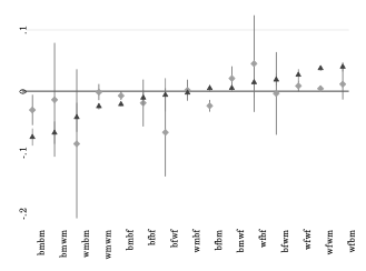
Prior to a discussion of these results, it is important to sound a caveat. These results are derived from changes in only a handful of cities and states and, as a result, the precision of some of these estimated effects may suffer. This is evident in some of the larger confidence intervals portrayed by the vertical bands in Figure 10 below.

With that in mind, the results presented here are quite interesting. To this point, regardless of how we slice the data (by region, politics, bank size, or intergroup proximity), we find that four groups of male same-sex loan co-applicants (black male/black male pairs, black male/white male pairs, white male/black male pairs and white male/white male pairs) are consistently discriminated against. These groups are approved for the same loans with the same income at the same banks in the same counties at lower rates. With the introduction of local antidiscrimination laws, a different picture emerges. Of the four disadvantaged groups, three are statistically indistinguishable from zero, meaning there is no evidence of discrimination in lending. The fourth group—a pair consisting of two black males—is still statistically significant and negative, meaning that that group is still less likely to have a loan approved, but the magnitude is smaller compared to the main results. In Table 7, a pair of two black males is 7.5 percentage points less likely to have a loan approved, all else equal. With the passage of a state or local antidiscrimination law, that rate drops in half to 3.1. The results suggest that state- and local-level attempts to discourage discrimination may be fruitful.243

To summarize, the analysis of the two potential mechanisms to discourage discrimination based on sexual orientation leads, at best, to mixed results. If population density is a good proxy for intergroup contact, we find no evidence that contact in more urbanized areas reduces the bias toward gay male couples. However, local attempts to enact laws designed to protect against sexual orientation discrimination may hold promise in reducing discrimination.

Conclusion

Discrimination in home mortgage lending has, unfortunately, a long history in the United States. Recent efforts to stave off discrimination in mortgage lending have included the creation of mortgage application databases to which lenders are required to report. Drawing on this data, the Article presents the first evidence of systematic, nationwide bias against perceived gay male applicants that transcends every geographical and political boundary in the United States. The data further suggests that prejudice, rather than statistical discrimination, is the driving force. The law has much to do with the current situation. With few exceptions, federal law and the majority of states do not prohibit lenders from discriminating against applicants based on their sexual orientation (although some localities do). In these jurisdictions, sexual orientation discrimination is not only legal, it is a defense that may allow a discriminatory lender to exculpate itself.

This study has important implications beyond the housing and mortgage lending markets. Sexual orientation discrimination has also been a burning topic in Title VII (employment) and Title IX (education) cases. In 2015, the same year in which the Supreme Court decided that the states are required to license and recognize same sex marriages,244 the EEOC held that Title VII’s prohibition against sex discrimination includes sexual orientation.245 That controversial decision was considered an outlier. For over half a century, the US Courts of Appeals resisted extending the prohibition against sex discrimination to sexual orientation.246 Although the Supreme Court has never spoken on the question, things may soon change.247 A few months ago, the Seventh Circuit, overruling previous precedents, held that sexual orientation discrimination is a form of sex discrimination and, therefore, is prohibited under Title VII.248 The decision sent shock waves throughout the legal community. And although the Seventh Circuit’s ruling was limited to Title VII purposes, it marks the beginning of a more dramatic change that may spread across jurisdictions and Titles.249

This Article can inform the ongoing debate over Title VII and other laws in pari materia. Indeed, with one exception,250 all US circuit courts now adopt and apply Title VII’s jurisprudence in mortgage lending.251 The same is true for the agencies in charge of enforcing the ECOA and FH Act.252

We end with an open invitation. Sexual orientation discrimination research is in its very early stages, with the first major study conducted overseas as late as 2009. We hope that our study will add to an important discussion that, to date, involves many theories but little empirical evidence. In that sense, a major contribution of our study is setting the grounds for a new form of econometric studies in the area.

• 1Telephone Interview with Ms. Renee Spears (Dec 30, 2017) (on file with authors); Rebekah Coleman, Gay Discrimination in the Mortgage Industry (Loans.org, Apr 12, 2013), archived at http://perma.cc/CC58-DRYG.
• 2See generally, for example, Obergefell v Hodges, 135 S Ct 2584 (2015) (holding that states cannot ban same-sex marriage); United States v Windsor, 570 US 744 (2013) (deciding that the Defense of Marriage Act’s definition of marriage as between a man and a woman was unconstitutional).
• 3Note that the “T” for transgender individuals is omitted. The reason is that courts have interpreted the prohibition against sex discrimination to also include discrimination against transgender applicants or, more broadly, gender identity discrimination. See Part I.A.1.
• 4We use the term “defense” here loosely to mean that the defendant was able to undermine the plaintiff’s ability to prove her case for unlawful discrimination. By contrast, an affirmative defense “is asserted only after the plaintiff establishes a prima facie case . . . against the defendant.” See Davenport v Cotton Hope Plantation Horizontal Property Regime, 508 SE2d 565, 571 (SC 1998) (comparing the defenses of implied primary and implied secondary assumption of risk).
• 5See notes 74–80 and accompanying text.
• 6For a partial list, see Ending Housing Discrimination against Lesbian, Gay, and Transgender Individuals and Their Families (Department of Housing and Urban Development), archived at http://perma.cc/77JP-JXCM.
• 7City of Ann Arbor Code, Ch 112, § 9:150 (defining discrimination as making a decision based on the “actual or perceived . . . sexual orientation . . . of another person or that person’s relatives or associates”).
• 8Atlanta, Ga, Ord Ch 94, Art IV, § 94–96 (prohibiting businesses engaged in residential real estate–related transactions from discriminating on the basis of actual or perceived sexual orientation). See also Cities & Counties with Non-discrimination Ordinances That Include Sexual Orientation (Human Rights Campaign, Jan 28, 2017), archived at http://perma.cc/6QU6-TRSR.
• 9See Ark Code Ann § 14-1-403 (“A county, municipality, or other political subdivision of the state shall not adopt or enforce an ordinance, resolution, rule, or policy that creates a protected classification or prohibits discrimination on a basis not contained in state law.”); Tenn Code Ann § 7-51-1802 (including a similar prohibition).
• 10Equal Access to Housing in HUD Programs Regardless of Sexual Orientation or Gender Identity, 77 Fed Reg 5662, 5662 (2012), codified at 24 CFR § 5 et seq (Equal Access Rule).
• 11Pub L No 94-200, 89 Stat 1125, (1975), codified as amended at 12 USC § 2801 et seq.
• 12In a joint mortgage application filed by two individuals, one is listed as the “primary” applicant and the other as a “secondary” applicant. In our baseline, the white male is the primary applicant and the white female is the secondary applicant—the most common combination in the dataset.
• 13See Kimberle Crenshaw, Demarginalizing the Intersection of Race and Sex, 1989 U Chi Legal F 139, 140 (explaining how courts’ failure to understand and properly analyze intersectional claims can leave subsets of protected groups—for example, black females—without a Title VII remedy, and warning that, “[b]ecause the intersectional experience is greater than the sum of racism and sexism, any analysis that does not take intersectionality into account cannot sufficiently address the particular manner in which Black women are subordinated”); Kimberle Crenshaw, Mapping the Margins: Intersectionality, Identity Politics, and Violence against Women of Color, 43 Stan L Rev 1241, 1244 (1991) (exploring “the various ways in which race and gender intersect in shaping structural, political, and representational aspects of violence against women of color”).
• 14See, for example, Nathanael Lauster and Adam Easterbrook, No Room for New Families? A Field Experiment Measuring Rental Discrimination against Same-Sex Couples and Single Parents, 58 Soc Probs 389, 401 (2011) (concluding, based on a field experiment, that “same-sex male couples saw the greatest rental discrimination . . . and were nearly 25 percent less likely to receive a positive response to a typical apartment inquiry” compared to heterosexual and same-sex female couples). In two different studies, Professors Ali Ahmed and Mats Hammarstedt found that gay couples are discriminated against in the rental market in Sweden (compared to heterosexual couples) but could not find a differential treatment between lesbian couples and heterosexual couples, suggesting that the discrimination was mainly against gay male couples. See Ali M. Ahmed and Mats Hammarstedt, Detecting Discrimination against Homosexuals: Evidence from a Field Experiment on the Internet, 76 Economica 588, 592 (2009); Ali M. Ahmed, Lina Andersson, and Mats Hammarstedt, Are Lesbians Discriminated against in the Rental Housing Market? Evidence from a Correspondence Testing Experiment, 17 J Housing Econ 234, 236–37 (2008). Similar findings—discrimination against gay male individuals but not lesbian individuals—were also documented in the labor market. See Ahmed, Andersson, and Hammarstedt, 17 J Housing Econ at 234, 236–37 (cited in note 14) (reviewing the literature on labor market discrimination against gay and lesbian individuals and finding that there is little evidence for labor market discrimination against lesbians); Bruce Elmslie and Edinaldo Tebaldi, Sexual Orientation and Labor Market Discrimination, 28 J Labor Rsrch 436, 436, 449–50 (2007) (finding that gay men face wage discrimination while lesbian women do not); Gregory M. Herek, Gender Gaps in Public Opinion about Lesbians and Gay Men, 66 Pub Op Q 40, 58 (2002) (“[A]ggregate attitudes tend to be more hostile toward gay men than lesbians.”).
• 15See Part II.C.2.
• 16Sexual Orientation and Housing Discrimination in Michigan: A Report of Michigan’s Fair Housing Centers *5 (Michigan’s Fair Housing Centers, Jan 30, 2007), archived at http://perma.cc/CC58-WSN6 (Michigan Study).
• 17See generally Lei Gao and Hua Sun, The Rainbow of Credit: Same-Sex Mortgage Discrimination and Two-Sided Spillover Effect (Iowa State University College of Business Working Paper, Apr 2017), archived at http://perma.cc/SGT5-MD4M.
• 18See Part I.D.3.
• 19In the Michigan Study, the couples posing as heterosexual and same-sex were of the same race. Similarly, Professors Lei Gao and Hua Sun tested the approval rate of all same-sex couples, controlling for race but not exploring the comparisons or interplay between race and sexual orientation. This design did not allow them to address the intersectionality question—how race and sex impact the approval rates—or to test how state and local rules impact these rates.
• 20See Equal Access Rule, 77 Fed Reg at 5662 (cited in note 10). See also Part I.A.3.
• 21See Part II.A.1.
• 22See Freedom from Discrimination in Credit Act, HR 2498, 115th Cong, 1st Sess, in 163 Cong Rec H 4310 (daily ed May 17, 2017). The Act would amend the Equal Credit Opportunity Act to prohibit sexual orientation discrimination in the provision of credit. Previous versions were introduced in 2009, 2011, 2013, and 2015.
• 23See Hively v Ivy Tech Community College of Indiana, 853 F3d 339, 341 (7th Cir 2017) (en banc) (holding that discrimination on the basis of sexual orientation is illegal sex discrimination under Title VII).
• 24See Philpott v New York, 252 F Supp 3d 313, 315 (SDNY 2017) (holding that a sexual orientation discrimination claim is “cognizable under Title VII”).
• 25See Franchina v City of Providence, 881 F3d 32, 54 (1st Cir 2018) (holding that a plaintiff may recover under a “sex-plus claim[ ] . . . where, in addition to the sex-based charge, the ‘plus’ factor is the plaintiff’s status as a gay or lesbian individual”).
• 26See Zarda v Altitude Express, Inc, 883 F3d 100, 112 (2d Cir 2018) (en banc) (holding that “sexual orientation discrimination is . . . a subset of sex discrimination”).
• 27See, for example, Equal Employment Opportunity Commission v R.G. & G.R. Harris Funeral Homes, Inc, 884 F3d 560, 574–75 (6th Cir 2018) (relying on the Seventh Circuit’s analysis in Hively in holding that “discrimination on the basis of transgender and transitioning status violates Title VII”); Wittmer v Phillips 66 Co, 304 F Supp 3d 627, 634 (SD Tex 2018) (adopting Zarda’s rationale and holding that “[t]he same is true for discrimination based on transgender status”); United States v Dental Dreams, LLC, 307 F Supp 3d 1224, 1253 (D NM 2018) (recognizing that sexual orientation discrimination is prohibited under Title VII).
• 28Pub L No 90-284, 82 Stat 81 (1968), codified as amended at 42 USC § 3601 et seq.
• 29Pub L No 93-495, 88 Stat 1521 (1974), codified as amended at 15 USC § 1691 et seq.
• 30See 42 USC § 3605(a):

  It shall be unlawful for any person or other entity whose business includes engaging in residential real estate-related transactions to discriminate against any person in making available such a transaction, or in the terms or conditions of such a transaction, because of race, color, religion, sex, handicap, familial status, or national origin.

  See also 15 USC § 1691(a) (“It shall be unlawful for any creditor to discriminate against any applicant, with respect to any aspect of a credit transaction . . . on the basis of race, color, religion, national origin, sex or marital status, or age (provided the applicant has the capacity to contract).”).

• 31See 42 USC §§ 3601–19; 15 USC § 1691.
• 32See 15 USC § 1691(a)(1) (making it unlawful to discriminate based on marital status or age); 42 USC § 3605(a) (prohibiting discrimination based on familial status and handicap).
• 33This interpretation may soon change. Many circuit courts view the ECOA and the FH Act as statutes in pari materia with Title VII, which is now interpreted by some courts as also protecting against sexual orientation discrimination. See notes 23–26. For circuits holding that Title VII jurisprudence applies in ECOA cases, see Wise v Vilsack, 496 Fed Appx 283, 285 (4th Cir 2012); Rosa v Park West Bank & Trust Co, 214 F3d 213, 215 (1st Cir 2000); Lewis v ACB Business Services, Inc, 135 F3d 389, 406 (6th Cir 1998). For circuits holding that Title VII jurisprudence applies in FH Act cases, see Gamble v City of Escondido, 104 F3d 300, 304 (9th Cir 1997); Larkin v Michigan Department of Social Services, 89 F3d 285, 289 (6th Cir 1996); Cabrera v Jakabovitz, 24 F3d 372, 383 (2d Cir 1994); Ring v First Interstate Mortgage, Inc, 984 F2d 924, 926 (8th Cir 1993); Doe v City of Butler, 892 F2d 315 (3d Cir 1989).
• 34See Equal Access Rule, 77 Fed Reg at 5668 (cited in note 10) (explaining that the FH Act “prohibits discrimination against someone who has or is regarded as having a disability, including HIV/AIDS”). For similar examples in the context of eviction from a rental property, see Memorandum for FHEO Reginal Directors regarding Assessing Complaints That Involve Sexual Orientation, Gender Identity, and Gender Expression *1 (Department of Housing and Urban Development, June 15, 2010), archived at http://perma.cc/LU6T-D965; Fact Sheet: Fair Housing for LGBT Persons *1 (Fair Housing Center of West Michigan), archived at http://perma.cc/D79Q-EXU9 (noting that the FH Act’s protection against housing discrimination on the basis of disability applies not only “to individuals with disabilities, but also to people who are regarded by others to have a disability whether or not they in fact have a disability”).
• 3542 USC § 3605(a).
• 3642 USC § 3602(h)(3).
• 37The Department of Housing and Urban Development (HUD) adopted a similar view. See generally Ending Housing Discrimination (cited in note 6).
• 38See notes 46–47 and accompanying text.
• 39490 US 228 (1989), superseded on other grounds by statute, Civil Rights Act of 1991, Pub L No 102-166, 105 Stat 1071, 1075-76, codified at 42 USC § 2000e–2(m).
• 40Id at 235.
• 41Id.
• 42Hopkins v Price Waterhouse, 618 F Supp 1109, 1117 (DDC 1985), affd in part, revd in part, 825 F2d 458 (DC Cir 1987), revd, 490 US 228 (1989).
• 43Price Waterhouse, 490 US at 235.
• 44See id at 250 (Brennan) (plurality) (stating that, “[i]n the specific context of sex-stereotyping, an employer who acts on the basis of a belief that a woman cannot be aggressive, or that she must not be, has acted on the basis of gender”). See also id at 258–61 (White concurring); id at 272–73 (O’Connor concurring).
• 45Smith v City of Salem, 378 F3d 566, 574 (6th Cir 2004). The extent of the protection, however, is still unclear. Some courts take the view that discrimination against a transgender plaintiff is unlawful only when it is based on gender stereotypes. See Etsitty v Utah Transit Authority, 502 F3d 1215, 1222, 1224 (10th Cir 2007) (holding that “transsexuals may not claim protection under Title VII from discrimination based solely on their status as a transsexual . . . [r]ather, [a transgender individual’s] claim must rest entirely on the Price Waterhouse theory of protection as a man who fails to conform to sex stereotypes,” and concluding that an employer is not “require[d] [ ] to allow biological males to use women’s restrooms”); Smith, 378 F3d at 575. Other courts have taken a more expansive approach, arguing that discrimination against transgender individuals is prohibited per se. See Glenn v Brumby, 663 F3d 1312, 1316 (11th Cir 2011) (“A person is defined as transgender precisely because of the perception that [their] behavior transgresses gender stereotypes.”); Macy v Holder, 2012 WL 1435995, *11 (EEOC) (“[I]ntentional discrimination against a transgender individual because that person is transgender is, by definition, discrimination ‘based on . . . sex,’ and such discrimination therefore violates Title VII.”). This also seems to be the view of the Consumer Financial Protection Bureau (CFPB). See Letter from Richard Cordray to Michael Adams and Aaron Tax, Application of the Equal Credit Opportunity Act to Credit Discrimination on the Bases of Gender Identity and Sexual Orientation *7 (Aug 30, 2016), archived at http://perma.cc/G6V6-YY47 (CFPB Letter) (relying on Title VII jurisprudence to conclude that “the prohibition of sex discrimination in ECOA and Regulation B affords broad protection against credit discrimination on the bases of gender identity and sexual orientation”). For a review of the two approaches, see generally Karen Moulding, 1 Sexual Orientation and the Law § 10:5 (Westlaw 2017).
• 46See Rosa, 214 F3d at 215 (discussed in notes 73–80).
• 47See Smith v Mission Association Ltd Partnership, 225 F Supp 2d 1293, 1299 (D Kan 2002) (“Sexual orientation claims are not actionable under the [FH Act].”).
• 48See Price Waterhouse, 490 US at 241–42. The plaintiff in these cases needs to show only that nonconformity with gender stereotypes was a consideration even if other considerations, such as the plaintiff’s sexual orientation, were also taken into account. See, for example, Centola v Potter, 183 F Supp 2d 403, 409 (D Mass 2002) (“[Plaintiff] does not need to allege that he suffered discrimination on the basis of his sex alone or that sexual orientation played no part in his treatment.”).
• 49See Price Waterhouse, 490 US at 241–42.
• 5015 USC §§ 1691–1691f; 12 CFR Part 1002.
• 51CFPB Letter at *4–7 (cited in note 45).
• 52Id at *4.
• 53The doctrine was adopted already in 1985 by the Federal Reserve in its official interpretation of Regulation B. 50 Fed Reg 48018, 48049 (1985). It was reaffirmed by the CFPB in the restated Regulation B. 76 Fed Reg 79442, 79473 (2011); 81 Fed Reg 25323, 25325 (2016); 12 CFR Part 1002, Supp I, § 2(z)-1:

  As used in this part, prohibited basis refers not only to characteristics—the race, color, religion . . . of an applicant . . . but also to the characteristics of individuals with whom an applicant is affiliated or with whom the applicant associates. This means, for example, that under the general rule stated in § 1002.4(a), a creditor may not discriminate against an applicant . . . because of the race of other residents in the neighborhood where the property offered as collateral is located.

  See also Interagency Policy Statement on Discrimination in Lending, 59 Fed Reg 18266, 18268 (1994) (“A lender may not discriminate on a prohibited basis because of the characteristics of: [a] person associated with a credit applicant.”).

• 54See CFPB Letter at *4 (cited in note 45).
• 55Unlike HUD, the CFPB does not provide any information about the number of complaints alleging discriminatory behavior. A search on its database yielded only a handful of discrimination-related claims, none of which seems to be in the mortgage lending context.
• 56See Equal Access Rule, 77 Fed Reg at 5662 (cited in note 10). See also generally Ending Housing Discrimination (cited in note 6).
• 57Equal Access Rule, 77 Fed Reg at 5662 (cited in note 10).
• 58See also generally Ending Housing Discrimination (cited in note 6).
• 59FHA Single Family Market Share *4 (Department of Housing and Urban Development, Apr 18, 2018), archived at http://perma.cc/52JA-WJD5 (providing statistics based on yearly activity and including purchased and refinanced loans). In 2009, the FHA market share peaked at 21.1 percent but remained at around 13 percent between 2012 and 2014.
• 60See id at *2.
• 61See Equal Access Rule, 77 Fed Reg at 5666 (cited in note 10) (refusing to interpret the FH Act as protecting against discrimination on the bases of sexual orientation and gender identity and explaining that the rule does not “create additional protected classes in existing civil rights laws”).
• 62See id at 5671.
• 63According to the National Fair Housing Alliance (NFHA), in 2016, only 28,181 complaints were filed nationwide for housing discrimination. Of these, 4.86 percent were processed by HUD, and only 150 complaints (0.01 percent) included sexual orientation discrimination claims. The Case for Fair Housing: 2017 Fair Housing Trends Report *79 (National Fair Housing Alliance, 2017), archived at http://perma.cc/QRK5-7MC3. The NFHA’s reports are available at http://nationalfairhousing.org/reports-research (visited Nov 27, 2018).
• 64853 F3d 339 (7th Cir 2017) (en banc).
• 65883 F3d 100 (2d Cir 2018) (en banc). Hively and Zarda, which held that sexual orientation discrimination is a subset of sex discrimination, were decided after the cases this Section references and mark a new trend. See notes 23–27, 248–49, and accompanying text. However, the early line of cases this Section discusses illustrate reasoning that could still come into play today in jurisdictions that have not adopted or explicitly rejected Hively and Zarda. See, for example, Bostock v Clayton County Board of Commissioners, 723 Fed Appx 964, 965 (11th Cir 2018) (adhering, per curiam, to prior Eleventh Circuit precedents foreclosing complaints for sexual orientation discrimination under Title VII).
• 66See notes 31–32.
• 67When a single motive guides the defendant’s decision, courts often apply the burden-shifting approach established in McDonnell Douglas Corp v Green, 411 US 792, 802–03 (1973). See also Husman v Toyota Motor Credit Corp, 12 Cal App 5th 1168, 1182–83 (2017) (explaining that, in mixed-motives cases, courts apply the Price Waterhouse framework). Under the McDonnell Douglas test, the plaintiff must first prove a discriminatory decision and offer facts suggesting the decision was based on an illegitimate motive. The burden then shifts to the defendant to show that the action had a legitimate motive. If the defendant meets the burden, the plaintiff must show that the lender’s reason is only pretextual or provide evidence of intentional discrimination. See also Dee Pridgen and Richard M. Alderman, Consumer Credit and the Law § 3:16 (Westlaw 2017) (noting that with the exception of the Seventh Circuit, “proof of discrimination in ECOA ‘disparate treatment’ suits will be subject to the analysis of McDonnell Douglas, as is the case with other discrimination claims, such as Title VII.”); Ring, 984 F2d at 926 (“We have no doubt that the three-stage McDonnell Douglas/Burdine analysis applies to Fair Housing Act cases.”).
• 68See also Price Waterhouse, 490 US at 251 (noting that mere remarks based on sex stereotypes do not prove that gender considerations guided the challenged decision; rather, “[t]he plaintiff must show that the [defendants] actually relied on her gender in making [their] decision”).
• 69The example is based on Rosa, 214 F3d 213. See notes 74–80 and accompanying text.
• 70See Part I.A.1.
• 71See, for example, Husman, 12 Cal App 5th at 1182–83 (discussing the burden-shifting procedures in single-motive and mixed-motives cases).
• 72Price Waterhouse, 490 US at 241.
• 73See id at 252 (holding that the defendant “must show that its legitimate reason, standing alone, would have induced it to make the same decision”). Under Price Waterhouse, such a showing fully exempted the defendant from liability. See id. This part of the decision, however, was short-lived. Two years later, Congress passed the Civil Rights Act of 1991, which severely limited the remedies available to a Title VII plaintiff but stopped short of immunizing the defendant from liability. See Harris v City of Santa Monica, 294 P3d 49, 57 (Cal 2013), quoting 42 USC § 2000e-5(g)(2)(B):

  [W]hen an individual “proves a violation” of Title VII and the [defendant] shows it “would have taken the same action in the absence of the impermissible motivating factor,” a court can “grant declaratory relief, injunctive relief . . . , and attorney’s fees and costs” directly attributable to the Title VII claim but “shall not award damages or issue an order requiring any admission, reinstatement, hiring, promotion, or payment. . . .”

  See also Husman, 12 Cal App 5th at 1184 (citing Harris with approval and noting that mixed-motives cases are not infrequent).

• 74214 F3d 213 (1st Cir 2000).
• 75Id at 214.
• 76Id.
• 77Id at 216.
• 78Rosa, 214 F3d at 215–16, citing Price Waterhouse, 490 US at 251 (“stereotyped remarks [including statements about dressing more ‘femininely’] can certainly be evidence that gender played a part.”).
• 79Rosa, 214 F3d at 215–16. The court reviewed the following possibilities:

  [1] It is reasonable to infer that Brunelle [the loan officer] told Rosa to go home and change because she thought that Rosa’s attire did not accord with his male gender. . . . If so, the Bank concedes, Rosa may have a claim. . . . [2] It is also reasonable to infer, though, that Brunelle refused to give Rosa the loan application because she thought he was gay, confusing sexual orientation with cross-dressing. If so, Rosa concedes, our precedents dictate that he would have no recourse under the federal Act. . . . [3] It is reasonable to infer, as well, that Brunelle simply could not ascertain whether the person shown in the identification card photographs was the same person that appeared before her that day. If this were the case, Rosa again would be out of luck. . . . [4] [F]inally [ ] Brunelle may have had mixed motives, some of which fall into the prohibited category.

  Id (citations omitted). Accordingly, the case was remanded to allow the parties to develop the evidence. Id.

• 80See id.
• 81Our focus is on members of the LGB community. See note 3. However, we refer to LGBT individuals when the discussion is also relevant to transgender individuals.
• 82398 F3d 211 (2d Cir 2005).
• 83Id at 218 (citation omitted), overruled by Zarda, 883 F3d 100.
• 84Dawson, 398 F3d at 218. For other Title VII decisions accepting the defendant’s sexual orientation discrimination defense, see Vickers v Fairfield Medical Center, 453 F3d 757, 763 (6th Cir 2006) (citing Dawson with approval); Simonton v Runyon, 232 F3d 33, 35–38 (2d Cir 2000) (en banc) (noting that the “[plaintiff]’s sexual orientation was known to his co-workers” and holding that Price Waterhouse’s sex stereotyping theory “would not bootstrap protection for sexual orientation into Title VII because not all homosexual men are stereotypically feminine, and not all heterosexual men are stereotypically masculine”), overruled by Zarda, 883 F3d 100; Ayala-Sepulveda v Municipality of San German, 661 F Supp 2d 130, 137 (D PR 2009) (citing Simonton with approval).
• 85183 F Supp 2d 403 (D Mass 2002).
• 86Id at 410.
• 87The court noted four separate times that the plaintiff did not reveal his sexual orientation at work. Id at 407, 410, 412.
• 88See id at 410. But see Dandan v Radisson Hotel Lisle, 2000 WL 336528, *4 (ND Ill) (rejecting the plaintiff’s claim that, “if the co-workers do not know his sexual orientation, the verbal abuse can only be attributed to the fact that he is a man” and explaining that “whether [defendant’s] co-workers knew or only suspected what his sexual orientation is makes no difference” because discrimination based on sexual orientation, real or perceived, is not actionable under Title VII). Still, disclosing the fact that one is a member of the LGB community may increase the likelihood not only of facing discrimination but also that a court would dismiss one’s sex discrimination claim in jurisdictions that have not followed Hively and Zarda.
• 89Centola, 183 F Supp 2d at 408.
• 90Prowel v Wise Business Forms, 579 F3d 285, 291 (3d Cir 2009) (vacating the lower court’s grant of summary judgment and “holding that [the plaintiff’s] sex discrimination claim was an artfully-pleaded claim of sexual orientation discrimination” because its analysis of “the facts and inferences in favor of [the plaintiff] leads [to the conclusion] that the record is ambiguous on this dispositive question”).
• 91Philpott, 252 F Supp 3d at 317.
• 92Id (quotation marks omitted).
• 93Centola, 183 F Supp 2d at 410.
• 94As we explain, this trend is changing. See notes 23–27, 248–49, and accompanying text.
• 95Vickers, 453 F3d at 763 (6th Cir 2006).
• 96Id (emphasis added). See also Dawson, 398 F3d at 221 (holding that “one can fail to conform to gender stereotypes in two ways: (1) through behavior or (2) through appearance” and dismissing the complaint after noting that the “[plaintiff] makes no assertion with respect to behavioral non-conformance”) (emphasis added), overruled by Zarda, 883 F3d 100.
• 97Glenn, 663 F3d at 1316. See also Macy, 2012 WL 1435995 at *9 (“A person is defined as transgender precisely because of the perception that [their] behavior transgresses gender stereotypes.”).
• 9842 USC § 3615 (stating that “[n]othing in this subchapter shall be construed to invalidate or limit any law of a State or political subdivision”).
• 9915 USC § 1691d(f) (“This subchapter does not annul, alter, or affect, or exempt any person subject to the provisions of this subchapter from complying with, the laws of any State with respect to credit discrimination, except to the extent that those laws are inconsistent with any provision of this subchapter.”).
• 100See note 9 and accompanying text.
• 101The asterisks denote that California, the District of Columbia, Vermont, and Wisconsin did not specify an effective date, and we assumed it was the same as the enactment date.
• 102This data about local level protections was collected using a number of databases, including Municode, Code Publishing, American Legal Publishing, General Code Corporation, Qcode, Coded Systems, and Conway Greene. See note 185.
• 103These studies are discussed in Part I.D.3.
• 104See notes 149–63 and accompanying text; Michigan Study (cited in note 16).
• 105See notes 156–59 and accompanying text. See generally Gao and Sun, The Rainbow of Credit (cited in note 17).
• 106Gary S. Becker, The Economics of Discrimination (Chicago 2d ed 1971).
• 107Id at 14–15.
• 108See Gary S. Becker, The Economic Approach to Human Behavior 17–19 (Chicago 1976). The reason for discrimination may also be the preference of a third party who is in a position to penalize those who decline to discriminate. See, for example, Cass R. Sunstein, Three Civil Rights Fallacies, 79 Cal L Rev 751, 754 (1991) (providing as examples “the case of a shopkeeper whose customers do not like dealing with blacks or women, a commercial airline whose patrons react unfavorably to female pilots, a law firm whose clients prefer not to have black lawyers, [and] a hospital whose patients are uncomfortable with female doctors or black nurses” and noting that, “[i]n [ ] these cases, an employer who introduces norms of equality into the work force will be punished, not rewarded”).
• 109Becker, Economic Approach to Human Behavior at 13–14 (cited in note 108).
• 110See id at 35–37.
• 111See id. See also Robert D. Cooter, The Strategic Constitution 340–41 (Princeton 2000); Richard H. McAdams, Relative Preferences, 102 Yale L J 1, 92–96 (1992) (reviewing the Becker model and offering an alternative theory of discrimination, claiming that discrimination may be the result of competition over social status between groups).
• 112See United Companies Lending Corp v Sargeant, 20 F Supp 2d 192, 203 n 5 (D Mass 1998) (“Redlining is the practice of denying the extension of credit to specific geographic areas due to the income, race, or ethnicity of its residents. . . . Reverse redlining is the practice of extending credit on unfair terms to those same communities.”).
• 113See Gary A. Dymski, Discrimination in the Credit and Housing Markets: Findings and Challenges, in William M. Rodgers III, ed, Handbook on the Economics of Discrimination 215, 220 (Edward Elgar 2006) (noting that the effects of racial preferences in a market depend on “the freedom of market entry, and on whether market participants face transaction and/or information costs”).
• 114See Gary A. Dymski, The Theory of Credit-Market Redlining and Discrimination: An Exploration, 23 Rev Black Political Economy 43–45 (Winter 1995) (explaining that discrimination may occur if the number of prejudicial lenders is large enough to dictate the price to the neutral lenders); Cooter, The Strategic Constitution at 344 (cited in note 111) (explaining that collusion by social groups can result in market power).
• 115See Kenneth Arrow, The Theory of Discrimination, in Orley Ashenfelter and Albert Rees, eds, Discrimination in Labor Markets 23–24 (Princeton 1973); Edmund S. Phelps, The Statistical Theory of Racism and Sexism, 62 Am Econ Rev 659, 660 (1972); Devin G. Pope and Justin R. Sydnor, What’s in a Picture? Evidence of Discrimination from Prosper.com, 46 J of Hum Res 53, 53 (Winter 2011) (“Accurate statistical discrimination is economically efficient for the decision maker, while taste-based discrimination stems from an animus toward one group and is often costly to the decision-maker.”).
• 116Hanmin Fang and Andrea Moro, Theories of Statistical Discrimination and Affirmative Action: A Survey, in Jess Benhabib, ed, 1A Handbook of Social Economics 135 (Elsevier 2011).
• 117Sunstein, 79 Cal L Rev at 755–56 (cited in note 108) (noting that “race or sex in some contexts may be every bit as accurate a predictor of job performance as, say, test scores, education, and previous employment” and that, “in some cases, reliance on more direct and individualized devices might be too costly to be worthwhile”).
• 118See United Companies, 20 F Supp 2d at 203 n 5.
• 119See Sunstein, 79 Cal L Rev at 755–57 (cited in note 108).
• 120See Jack M. Guttentag and Susan M. Wachter, Redlining and Public Policy 11–12 (NYU 1980).
• 121See, for example, id at 40–42 (saying that, because most redlining is rational, the costs of implementing antiredlining regulations do not justify the benefits.).
• 122See, for example, McAdams, 102 Yale L J at 91–96 (cited in note 111) (explaining that discrimination may be the result of competition over social status between groups).
• 123For studies drawing similar distinctions, see Lauster and Easterbrook, 58 Soc Probs at 391 (cited in note 14) (studying sexual orientation discrimination in the Canadian rental market); Uri Gneezy, John List, and Michael K. Price, Toward an Understanding of Why People Discriminate: Evidence from a Series of Natural Field Experiments *12–13 (National Bureau of Economic Research Working Paper No 17855, Feb 2012), archived at http://perma.cc/6LAW-U9M8 (studying discrimination in a number of service and product markets related to the automobile industry); Pope and Sydnor, 46 J Hum Res at 55–56 (cited in note 115) (studying discrimination in peer-to-peer lending markets).
• 124See Gordon W. Allport, The Nature of Prejudice 281 (Addison-Wesley 1954); Richard Delgado, et al, Fairness and Formality: Minimizing the Risk of Prejudice in Alternative Dispute Resolution, 1985 Wis L Rev 1359, 1382; Lauster and Easterbrook, 58 Soc Probs at 391 (cited in note 14).
• 125See generally Stephen L. Ross and Margery Austin Turner, Housing Discrimination in Metropolitan America: Explaining Changes between 1989 and 2000, 52 Soc Probs 152 (2005) (suggesting that a landlord may discriminate against members of a minority group based on such information).
• 126See Alicia H. Munnell, et al, Mortgage Lending in Boston: Interpreting HMDA Data, 86 Am Econ Rev 25, 32 (1996).
• 127See id at 33.
• 128See Raphael W. Bostic, The Role of Race in Mortgage Lending: Revisiting the Boston Fed Study *19–21 (Federal Reserve Board of Governors Division of Research & Statistics Working Paper, Dec 1996) (on file with authors). See generally Judith A. Clarke, Nilanjana Roy, and Marsha J. Courchane, On the Robustness of Racial Discrimination Findings in Mortgage Lending Studies, 41 Applied Econ 2279 (2009).
• 129See Peter Brimelow and Leslie Spencer, The Hidden Clue, Forbes (Jan 4, 1993) (suggesting that the observation used by Professor Alicia Munnell to justify discounting differences in default rates between races—the fact that there were no differences in default rates across census tracts that were populated by different racial groups—was recursive insofar as the minority borrowers in those census tracts had presumably already been filtered through a lender who predicted higher default rates among minorities).
• 130See Geoffrey M.B. Tootell, Redlining in Boston: Do Mortgage Lenders Discriminate against Neighborhoods?, 111 Q J Econ 1049, 1050–51 (1996).
• 131See Parts II.A–B.
• 132For example, we are able to limit the possibility of statistical discrimination by restricting the dataset to only FHA loans. Once issued, these loans carry the same risk to the bank regardless of any underlying characteristic that banks think they may need to account for that is associated with race, or sexual orientation. We also compare changes in lending rates by minority groups from the same bank in the same county.
• 133Pair Testing and the Housing Discrimination Studies (Department of Housing and Urban Development, Spring/Summer 2014), archived at http://perma.cc/652L-CVE6.
• 134Id.
• 135See, for example, Lauster and Easterbrook, 58 Soc Probs at 390 (cited in note 14) (“Much has been written about discrimination in the rental market, but the literature is almost entirely focused on race and ethnicity.”).
• 136See Ahmed and Hammarstedt, 76 Economica at 595 (cited in note 14) (“These results reveal that homosexual males were discriminated [against] since the homosexual couple in the study got fewer call-backs, fewer invitations to further contacts and fewer invitations to showings than the heterosexual couple.”).
• 137See id at 594.
• 138See Lauster and Easterbrook, 58 Soc Probs at 403 (cited in note 14). The author found that, compared to the heterosexual baseline, male couples were 24 percent less likely to receive a positive response to a rental inquiry. By contrast, lesbian couples were actually more likely to receive a positive response to rental inquiries than the heterosexual couple, though the effect was statistically insignificant. Id. The study also found support for the Contact Theory. In areas where individuals were more likely to have contact or familiarity with same-sex couples (for example, downtown), landlords “demonstrate[d] much less discrimination against same-sex male couples.” (The authors noted, however, that these areas were also the more expensive ones.) See id.
• 139See id at 398; Ahmed and Hammarstedt, 76 Economica at 592 (cited in note 14).
• 140For example, a discriminating landlord could, hypothetically, respond positively to the inquiry from the homosexual couple but make it difficult for the couple to actually see the apartment. Examples of this in practice may look like scheduling a visit multiple weeks out at an inconvenient time or requesting a phone conversation to confirm a date and time to tour the facility and never answering the phone.
• 141See Lauster and Easterbrook, 58 Soc Probs at 402 (cited in note 14).
• 142Samantha Friedman, et al, An Estimate of Housing Discrimination against Same-Sex Couples *2 (Department of Housing and Urban Development, June 2013), archived at http://perma.cc/5KXM-T6YZ. Although the HUD study was conducted in 2011 before the Equal Access Rule was promulgated, it was released to the public in July 2013.
• 143Id at *iv.
• 144Id at *6.
• 145See id at *vi (“[H]eterosexual couples were favored over gay male couples in 15.9 percent of tests and over lesbian couples in 15.6 percent of tests.”).
• 146See Friedman, et al, An Estimate of Housing Discrimination at *iv, vi–vii, 16–17.
• 147See Gneezy, List, and Price, Toward an Understanding at *16 (cited in note 123) (focusing on car dealerships in the Chicago area).
• 148See Friedman, et al, An Estimate of Housing Discrimination at vii (cited in note 142) (“The study measured the response of housing providers regarding the sexual orientation of couples and did not examine other characteristics.”); Gneezy, List, and Price, Toward an Understanding at *17 (cited in note 123).
• 149For an explanation of the methodology and its limitations, see Pair Testing and the Housing Discrimination Studies (cited in note 133) (“Much of the research into housing discrimination . . . relies on paired testing, a methodology in which two testers assume the role of applicants . . . who differ only in terms of the characteristic being tested for discrimination, such as race.”).
• 150Michigan Study at *3 (cited in note 16).
• 151Id at *9–10.
• 152Id.
• 153Id at *9.
• 154Michigan Study at *9 (cited in note 16).
• 155Id at *11.
• 156See generally Gao and Sun, The Rainbow of Credit (cited in note 17).
• 157Id at *4. The rate increased to 8 percent when conducted on the Boston Fed Dataset, “which includes an extensive list of property, neighborhood, borrower, and lender characteristics for a random sample of borrowers in Boston in 1990.” Id.
• 158Id.
• 159Id at *24.
• 160In the Michigan Study, like in other experiments, in each of the paired tests, the couples posing as same-sex couples and heterosexual couples were always of the same race. See Michigan Study at *3 (cited in note 16). Of these couples, the vast majority—113 (or 94 percent)—were white, five were black, and two were inter-racial. See id at *10. Gao and Sun controlled for race in their study but did not explore its interaction with sexual orientation in this context. See generally Gao and Sun, The Rainbow of Credit (cited in note 17).
• 161See Michigan Study at *9, 11 (cited in note 16) (admitting that “[m]ore testing is needed to see how the race and sex of testers [that is, of applicants] are influencing factors in some housing markets”).
• 162See id at *9 (“It is unclear whether [levels of discrimination found across the state diverged widely] due to differences in . . . the presence of local ordinances protecting sexual orientation.”). Although inconclusive, the Michigan Study reported that there was less evidence of discrimination in areas with such local ordinances (22 percent compared to 30 percent in areas without ordinances). See id at *16.
• 163Id at *9. The Swedish, Canadian, and HUD studies also suffer from this limitation. See generally Ahmed and Hammarstedt, 76 Economica 588 (cited in note 14).
• 164Gao and Sun, The Rainbow of Credit at *4 (cited in note 17).
• 165See notes 211–12 and accompanying text.
• 166These include the standards promulgated by the CFPB under the Ability-to-Repay and Qualified Mortgage Standards under the Truth in Lending Act (Regulation Z), 78 Fed Reg 35430, 35438–39 (2013), 12 CFR Part 1026, the FHA loan requirements discussed at http://www.fhahandbook.com (visited December 17, 2018), and additional requirements set by lenders and investors (known as “overlays”).
• 167See notes 202–03 and accompanying text.
• 168The “serious delinquency rate[ ],” defined as the “sum of 90-day delinquencies plus in-foreclosures and in-bankruptcies,” has been steadily reduced in recent years from 15.78 percent in 2007 to 0.05 percent in 2017. See FHA Single Family Loan Performance Trends *2 (Department of Housing and Urban Development, Feb 2017), archived at http://perma.cc/B24F-Y6PU.
• 169See Laurie S. Goodman, Quantifying the Tightness of Mortgage Credit and Assessing Policy Actions, 37 BC J L & Soc Just 235, 246 (2017) (reporting that in 2015 the annual cost of servicing performing loans was $181 compared to $2,386 for nonperforming loans).
• 170See 12 USC § 1708(c)(3); 24 CFR § 25.2 (“The Board has the authority to take any administrative action against mortgagees and lenders.”); 24 CFR § 25.5 (giving the board the power to issue “a letter of reprimand, probation, suspension, or withdrawal; or enter into a settlement agreement.”).
• 171HUD’s Mortgagee Review Board (MRB) “is empowered to initiate the issuance of a letter of reprimand, the probation, suspension or withdrawal of any mortgagee found to be engaging in activities in violation of [FHA] requirements or the nondiscrimination requirements of the [ECOA], the [FH Act], or Executive Order 11063.” 12 USC § 1708(c)(1). See also 24 CFR § 25.5 (detailing the effect of these administrative actions). The MRB is also authorized “to impose civil money penalties upon mortgagees and lenders.” See 24 CFR § 25.2(b)(2); 24 CFR § 30.15; 24 CFR § 30.35(b)–(c)(1) (“Each day that a violation continues shall constitute a separate violation” for which “[t]he maximum penalty is $9,819 . . . up to a limit of $1,963,870 for all violations committed during any one-year period.”).
• 172See Bernadette Kogler, Ann Schnare, and Tim Willis, Lender Perspectives on FHA’s Declining Market Share *25 (Research Institute for Housing America, Aug 2006), archived at http://perma.cc/5DCV-RE5H (explaining that HUD can “require a lender to ‘indemnify’ the department” when the “insured loan [ ] was not originated in compliance with FHA guidelines,” and reporting that “interviews revealed that HUD indemnifications result from comparatively minor documentation deficiencies that are not necessarily related to a borrower’s ability or willingness to repay”).
• 173A major source of concern for lenders is the False Claims Act (FCA), Pub L No 97-258, 96 Stat 978 (1982), codified as amended at 31 USC § 3729 et seq. The FCA allows the government to recover from those who knowingly make a false record or submit a fraudulent claim three times the damages sustained by the government. See 31 USC § 3729(a)(1). Because FHA lenders must certify their compliance with HUD’s rules, they are exposed to FCA litigation for errors committed during the origination phase. See Goodman, 37 BC J L & Soc Just at 245 (cited in note 169) (arguing that “the big issue for FHA servicers is the presence of the False Claims Act” and noting that, in 2016, settlements with lenders for FCA violations were close to $5 billion).
• 174See Kolger, Schnare, and Willis, Lender Perspectives at *24–25 (cited in note 172) (reporting that, in a study completed by sixty-one lending institutions, negative publicity was “cited as a moderate or minimal risk by most respondents”).
• 175In fact, there is some evidence to the contrary. See, for example, The LGBT Financial Experience: 2012–2013 Prudential Research Study *10 (Prudential, 2013), archived at http://perma.cc/RU4W-6MZH (“The LGBT community has a higher median income compared to the general population” and a “high discretionary income, with 40% of gay men and 25% of lesbians spending more than $500 a month on discretionary items.”). See also Gao and Sun, The Rainbow of Credit at *24 (cited in note 17) (concluding that “same-sex status exhibits no greater risk of default,” that “there is no evidence that same-sex borrowers are riskier for lenders, and [that some findings] suggest that it may be the opposite”). Moreover, Gao and Sun find that “HMDA estimation without extensive controls on borrower’s characteristics [such as creditworthiness] seems to provide a conservative lower bound on the magnitude of lending discrimination to same-sex borrowers.” Id at *4 (emphasis added).
• 176One possible concern could be that county data is not granulated enough to capture the self-selection dynamic that may take place in certain neighborhoods within the same county. The reason is that some counties have neighborhoods that vary dramatically in terms of their default risk. Thus, if same-sex couples are more likely to take a risk on being an early entrant into a transitioning neighborhood, they may pose a higher risk to the lender, but this may not show in county-level data. Here it is important to note that, while our main results are reported using bank-by-county fixed effects, the results are insensitive to using census tract–by–bank fixed effects, which can address such potential selection effects. We also address this concern (although for a different purpose) by comparing mortgages within counties in other regions in the United States—particularly in rural counties. In these regions, the concern that there is unobserved variation in risk due to self-selection within county is mitigated. We find that the results hold when looking exclusively at rural counties. See note 232 and accompanying text.
• 177See, for example, Joshua J. Miller and Kevin A. Park, Same-Sex Marriage Laws and Demand for Mortgage Credit *8, 20 (Department of Housing and Urban Development Working Paper No HF-020, Feb 2016), archived at http://perma.cc/9PFY-FM8R (estimating, based on the reported sex of co-applicants, that states that passed same-sex marriage laws experienced an 8 to 13 percent increase in mortgage applications).
• 178See notes 39–44 and accompanying text.
• 179A parent and child may both be gay individuals or may be perceived as such by the loan officer. It could also be that one of them is a gay individual (that is, the parent or the child may be a gay individual).
• 180135 S Ct 2584 (2015). See generally Miller and Park, Same-Sex Marriage Laws (cited in note 177).
• 181Miller and Park, Same-Sex Marriage Laws at *1 (cited in note 177).
• 182Id at *2.
• 183The vertical axis measures proportions for each series separated on the horizontal axis into each state and the District of Columbia.
• 184Data on the LGBT community comes from Same-Sex Couple and LGBT Demographic Data Interactive (The Williams Institute, UCLA School of Law, May 2016), archived at http://perma.cc/A9T7-LXPM.
• 185All state-level fair housing laws were collected from Westlaw. For states that had sexual orientation protection, we recorded the date the statute was passed or the relevant section was added and the date it became effective. Assembling a database that includes all local and county ordinances was more challenging. First, no one source compiles all local laws. In addition, we found that some localities maintain extensive histories, while others do not. To address these issues, we reviewed a number of leading databases, including Municode, Code Publishing, American Legal Publishing, General Code Corporation, Qcode, Coded Systems, and Conway Greene. We then compared the results to earlier lists by other organizations, such as the Human Rights Campaign, and attempted to track the legislative history—particularly the enactment and effective dates—for ordinances with sexual orientation protection.
• 186We chose these years in an attempt to avoid the housing market crash and aftermath.
• 187A similar method is employed in a study of FHA loans that did not require co-applicants by Greg Buchak and Adam Jørring, Does Competition Reduce Racial Discrimination in Lending? *7 (unpublished research paper, The University of Chicago, 2016), archived at http://perma.cc/YB9F-BHM6.
• 188This measurement of loan application success is a common measure in the discrimination literature. See, for example, id at *11.
• 189There are three property types: single family, multifamily, and manufacturing housing.
• 190The “loan purpose” can be home purchase, home improvement, or home refinancing.
• 191For instance, the changing landscape of home mortgages in the United States following the housing market collapse would be accounted for with year-fixed effects.
• 192With the HMDA dataset, we are able to drill down to a geographical level of granularity finer than county and go all the way down to census tract, which typically consists of neighborhoods within a county with a population of around four thousand. For computational reasons, we feel county-by-bank effects are more appropriate. One major empirical decision to balance in this Article is the tradeoff between very precise data and allowing for enough identifying variation. For instance, if we compared the same banks within a state, that would provide plenty of observations nested within each fixed effect, but it may oversimplify the mortgage process because geographic and economic conditions vary wildly within a state. On the other hand, drilling down to the neighborhood level provides the best comparison, but functionally, the analysis is weakened by the lack of diversity in application types. Put differently, if we compare Bank A in State 1, there will be lots of applications to look at, but they will be for homes in potentially very different neighborhoods. On the other hand, if we look only in the same neighborhoods, there is a real possibility that a bank may not cover all fifteen types of race/gender combinations we analyze in this study. We believe that county-by-bank effects best balance the need for a tight comparison window while keeping a critical mass of observations in each window. The main results are, however, completely unchanged if we instead include census tract–by–bank effects.
• 193See notes 188–90 and accompanying text.
• 194See Miller and Park, Same-Sex Marriage Laws at *6 (cited in note 177).
• 195See generally William Greene, The Behaviour of the Maximum Likelihood Estimator of Limited Dependent Variable Models in the Presence of Fixed Effects, 7 Econometrics J 98 (2004).
• 196See Gary King and Langche Zeng, Logistic Regression in Rare Events Data, 9 Political Analysis 137, 150 (2001).
• 197For a defense of such studies, see generally James H. Carr and Isaac F. Megbolugbe, The Federal Reserve Bank of Boston Study on Mortgage Lending Revisited, 4 J Housing Rsrch 277 (1993); Lynn E. Browne and Geoffrey M.B. Tootell, Mortgage Lending in Boston—A Response to the Critics, 1995 New England Econ Rev 53.
• 198See The LGBT Financial Experience at *10 (cited in note 175).
• 199For computation reasons, we include county-by-bank fixed effects. Our results are insensitive to the inclusion of census tract–by–bank fixed effects, which is an even more direct measure of neighborhood effects.
• 200We add a word of caution. Although our findings suggest that the discrimination is motivated by bigotry, it is important to note that other forces may be in play that may explain the results. First, the discrimination observed may be the result of “carried-over” discrimination—that is, discrimination that occurred prior to the application process, and what we observe in the mortgage market is just a downstream consequence of previous discrimination. For example, if members of the LGB community are discriminated against in labor markets and consequently switch jobs more often than other groups, they may be less likely to be approved for FHA loans, which require that applicants hold a steady two-year income. In this regard, we are able to control for loans that were denied due to employment history, so any observed discriminatory effect is occurring independent of upstream employment discrimination. LGB individuals may also find it harder to meet the FHA documentation requirement. One recent study reports that 57 percent of LGBTQ individuals experienced discrimination across many areas of life.” See Discrimination in America: Experiences and Views of LGBTQ Americans *2 (NPR, Nov 2017), archived at http://perma.cc/FV28-9GZJ. Another reports that “34% of LGBT people who experienced discrimination in the past year avoided public places . . . and 18% avoided doctors’ offices.” Movement Advancement Project, LGBT Policy Spotlight: Public Accommodations Nondiscrimination Laws *2 (MAP, 2018), archived at http://perma.cc/EV8H-FMM5. Combined, these studies suggest that members of the LGBT community are less likely to produce necessary documents. Similar to employment history, we are able to control for applications that were denied due to improper documentation. Moreover, the observed discrimination may be, at least in part, the product of other agents. For example, the discrimination may be due to disparate treatment by bigoted appraisers who are required to assess the purchased property. However, taken together, it is more likely that discrimination takes place at the point of sale—that is, with the loan officer.
• 201See note 168.
• 202For a recent article employing a similar strategy, see generally Buchak and Jørring, Does Competition Reduce Racial Discrimination? (cited in note 187).
• 203See id at *7–8.
• 204Columns (1) and (2) in this table each represent a unique regression in which the unit of observation is at the individual loan application level. Column (1) includes year-fixed and county-by-bank fixed effects, and Column (2) includes the same fixed effects plus the other controls mentioned in the text. Each row represents the marginal effect of the probability of a loan getting accepted for the associated pairing of applicant and co-applicant where the comparison group is a white male applicant with a white female co-applicant. Robust standard errors clustered at the state level are reported below in parentheses. Statistical significance levels are marked as * p<0.10, ** p<0.05, *** p<0.01.
• 205See notes 188–91 and accompanying text.
• 206This figure displays graphically the empirical results from Column (2) in Table 2. The marginal effect for each gender and race combination is measured on the vertical axis, and each combination of race and gender is measured on the horizontal axis. The first letter in each horizontal axis label represents the race of the applicant, the second letter signifies the gender, the third letter represents the race of the co-applicant, and the last letter represents the gender of the co-applicant. For example, “bmbm” stands for a black male applicant with a black male co-applicant. In this specification and all other specifications, we make no assumption about the symmetry of an applicant and co-applicant. That is, there might be reason to believe wmbm may be treated differently from the symmetric pairing, bmwm, so we treat each as different. This allows us to check if there is a “primary applicant” or “secondary applicant” effect.
• 207Part II.A.2 reports two additional robustness tests. See notes 183–93 and accompanying text.
• 208Group 2 relationships are ambiguous to the lender. See note 179 and accompanying text.
• 209See Buchak and Jørring, Does Competition Reduce Racial Discrimination? at *14 (cited in note 187).
• 210See id (7 percentage points); Munnell, et al, 86 Am Econ Rev at 33 (cited in note 126) (8.2 percentage points).
• 211See generally Friedman, et al, An Estimate of Housing Discrimination (cited in note 142) (finding a similar, but larger, effect for gay men compared to lesbian women); Lauster and Easterbrook, 58 Soc Probs at 389 (cited in note 14) (finding an even more pronounced discrimination against gay men).
• 212See, for example, Robert Anderson and Tina Fetner, Cohort Differences in Tolerance of Homosexuality: Attitudinal Change in Canada and the United States, 72 Pub Opinion Q, 311, 314 (2008); Gregory M. Herek and John P. Capitanio, Sex Differences in How Heterosexuals Think about Lesbians and Gay Men: Evidence from Survey Context Effects, 36 J Sex Rsrch 348, 357 (1999). See also Elmslie and Tebaldi, 28 J of Labor Rsrch at 441 (cited in note 14) (a labor market study noting that “[t]he bias against gay men is much stronger than the bias toward lesbians”).
• 213See Part II.A.2 and notes 207–08 and accompanying text.
• 214For more on census regions, see Geographic Terms and Concepts—Census Divisions and Census Regions (United States Census Bureau), archived at http://perma.cc/S64H-9443.
• 215Unlike in Table 2, each column in Table 3 reports results for the same regression that splits the effect of each race and gender pairing by region. This regression includes all the same controls and fixed effects as Column (2) of Table 3, and the standard errors are clustered at the state level. While we do not report the results by region without controls similar to Column (1) of Table 2, the results are available upon request and are virtually the same as the results that Table 3 reports. Statistical significance levels are marked as * p<0.10, ** p<0.05, *** p<0.01.
• 216While the interpretation of the intervals and the points in the intervals is the same as in Figure 4, it is important to note that each region subfigure in Figure 6 is derived from the same regression—which Table 4 reports—aimed to tease out regional effects in discrimination based on sexual orientation.
• 217Formal statistical tests of equivalence across regions suggests that of the fifteen combinations of race and gender, only five are statistically different—suggesting again that in most cases, there is very little difference in the effects across regions.
• 218Those states are California, Connecticut, Delaware, Hawaii, Illinois, Maine, Maryland, Massachusetts, New Jersey, New Mexico, New York, Oregon, Rhode Island, Vermont, and Washington.
• 219Alabama, Alaska, Arizona, Arkansas, Georgia, Idaho, Indiana, Kansas, Kentucky, Louisiana, Mississippi, Missouri, Montana, Nebraska, North Dakota, Oklahoma, South Carolina, South Dakota, Tennessee, Texas, Utah, Wyoming, and West Virginia.
• 220Colorado, Florida, Iowa, Michigan, Minnesota, Nevada, New Hampshire, North Carolina, Ohio, Pennsylvania, Virginia, and Wisconsin. These characterizations are based on the outcomes of previous presidential elections as reported by www.270towin.com, though the results are insensitive to alternative specifications of swing states.
• 221This Table is organized in the same manner as Table 5. Each column includes estimates for each applicant/co-applicant pairing from the same regression that includes all the controls and fixed effects. Each column also clusters the robust standard errors at the state level. Statistical significance levels are marked as * p<0.10, ** p<0.05, *** p<0.01.
• 222This Figure replicates the results that Figure 6 presents in every way except when each coefficient is split by party lines instead of region. Additionally, the main result from Figure 2 is included in the top left quadrant by way of comparison.
• 223In our dataset, those banks include loandepot.com, Flagstar Bank, Freedom Mortgage, Advanced Financial Services, JP Morgan Chase, Quicken Loans, Bank of America, and three different classifications for Wells Fargo.
• 224In this table, each race and gender pairing was sorted by whether the application went to a “big bank,” medium bank, or a smaller bank. The results in this table are generated by the same regression and are organized similarly to the previous two tables. Statistical significance levels are marked as * p<0.10, ** p<0.05, *** p<0.01.
• 225Both subfigures come from a single regression that Table 6 reports. This figure reads and interprets the same as each previous figure.
• 226For a review of intergroup bias and attempts to decrease it, see Thomas F. Pettigrew and Linda R. Tropp, A Meta-analytic Test of Intergroup Contact Theory, 90 J Personality and Soc Psychology 751, 766–83 (2006).
• 227As an example, see generally Shana Levin, Colette van Laar, and Jim Sidanius, The Effects of Ingroup and Outgroup Friendships on Ethnic Attitudes in College: A Longitudinal Study, 6 Group Processes & Intergroup Relations 76 (2003) (finding that college students exposed to intergroup relationships were more likely to report having friends from those groups and less likely to display biased behaviors in subsequent college years).
• 228See David Broockman and Joshua Kalla, Durably Reducing Transphobia: A Field Experiment on Door-to-Door Canvassing, 352 Science 220, 223 (2016).
• 229Consider Briggs Depew and Isaac D. Swensen, The Decision to Carry: The Effect of Crime on Concealed-Carry Applications (IZA Institute of Labor Economics Discussion Paper No 10236, Sept 2016), archived at http://perma.cc/MEJ5-JYB7. This Article splits groups between rural and urban in a similar fashion.
• 230See Tables 3 through 5 for more information on interpreting this table.
• 231This Figure reports the regression results of Table 3. See Figure 2 for more details on the construction and interpretation of this Table.
• 232The groups are (i) black male pairs (experiencing the most discrimination), followed by (ii) black male/white male pairs, then (iii) white male/black male pairs, and finally (iv) white male pairs.
• 233The Equal Access Rule, which prohibits lenders of FHA loans from engaging in this form of discrimination, is an administrative rule. As HUD explicitly admits, the Rule does not create a new right for aggrieved parties. See Equal Access Rule, 77 Fed Reg at 5670–71 (cited in note 10).
• 234See Part I.C.
• 235Yuval Feldman and Orly Lobel, The Incentives Matrix: The Comparative Effectiveness of Rewards, Liabilities, Duties, and Protections for Reporting Illegality, 88 Tex L Rev 1151, 1184 (2010).
• 236As a hypothetical, imagine a variable called “tolerance toward the LGB community.” If this were a variable we could measure, we might find that this variable is highly correlated with the passage of local laws prohibiting sexual orientation discrimination. That is, localities that are more tolerant toward the LBG community may be more likely to pass laws protecting LGB individuals. The “tolerance toward the LBG community” variable would most likely also be correlated with our outcome of interest in our regressions: the probability of getting a loan approved for a perceived gay couple. Thus, if we were to just compare loan acceptance rates from (state and local) jurisdictions with laws protecting LGB individuals to jurisdictions without such laws, we might misinterpret any difference as caused by the law when, in fact, the driving force of the difference is not the law but rather the “tolerance toward the LGB community” variable.
• 237This is the case because states with these laws are probably fundamentally different from states without them.
• 238For the appropriate use of difference-in-differences estimators, see generally Marianne Bertrand, Esther Duflo, and Sendhil Mullainathan, How Much Should We Trust Differences-in-Differences Estimates?, 119 Q J Econ 249 (2004).
• 239Specifically, to calculate the second difference, the regression first focuses on jurisdictions that did not adopt a local law. For each of these jurisdictions, it compares the second difference: the acceptance rate before and after the effective date. The regression then compares the first difference (the acceptance rate in Nevada in the period between 2011 and 2015 minus the acceptance rate in Nevada in 2010) to the second difference (acceptance rate in all jurisdictions that did not adopt such laws for the period of 2011 to 2015 minus all the acceptance rates in these states in 2010). Formally, this technique requires the inclusion of group fixed effects that flag the treated local and state jurisdictions, a time-fixed effect that flags the treated time, and an interaction between the two.
• 240One of the assumptions of this modeling technique, however, is that the treated state or locality—that is, the jurisdiction that passed a law in our time window—looked much like the jurisdictions that serve as controls prior to the passage of the law in terms of the outcome variables—in our case, mortgage loan approvals. This assumption is necessary for valid inference. See Griffin Edwards, et al, Looking Down the Barrel of a Loaded Gun: The Effect of Mandatory Handgun Purchase Delays on Homicide and Suicide *14, (University of Alabama Legal Studies Research Paper No 2629397, 2017), archived at http://perma.cc/YM24-YHHS (“As is often the case with any policy passed by legislators, there is concern that the laws were passed endogenously to the outcome variable. We alleviate this concern as much as possible . . . by including controls that capture the political atmosphere of each state.”). In the context of our study, we compare what happened to perceived LGB couples in treated jurisdictions before the law changed and find that they looked very similar to the control states.
• 241In this table, each column represents the difference-in-differences estimate of the effect of the passage of a state law for each applicant/co-applicant pairing. Like other tables, this regression, estimated at the individual loan application level, includes fixed effects for year, bank-by-county, and all other controls included in each regression. Additionally, this regression includes group-fixed effects and a state/locality law time effect to capture the difference-in-differences estimator. Statistical significance levels are marked as * p<0.10, ** p<0.05, *** p<0.01.
• 242Each difference-in-differences estimator of the effect of the passage of a state anti–sexual orientation discrimination law on each race/gender group is represented by the diamond dots. The bands represent confidence intervals for the difference-in-differences estimates. By way of comparison, we have also included the baseline estimates from Figure 7 with triangle dots and corresponding confidence intervals. The bands represent confidence intervals. For more information on how to interpret this graph, see the previous figures.
• 243As we explain earlier, however, the results should be taken with caution given that they are derived from changes in laws in only a few states and localities.
• 244See generally Obergefell, 135 S Ct 2584.
• 245See generally Baldwin v Foxx, 2015 WL 4397641 (EEOC).
• 246See Brief for the United States as Amicus Curiae Supporting Appellees, Zarda v Altitude Express, No 15-3775, *7 (2d Cir filed July 26, 2017) (available on Westlaw at 2017 WL 3277292) (DOJ Brief) (“[U]ntil the Seventh Circuit’s en banc decision in Hively earlier this year, the ten other Courts of Appeals to have addressed the issue had uniformly joined this Court in holding that Title VII’s prohibition on sex discrimination does not encompass sexual orientation discrimination.”).
• 247On May 29, 2018, the defendant-employer in Zarda filed a petition for writ for certiorari, asking the Supreme Court to reverse the Second Circuit’s decision and hold that Title VII does not prohibit sexual orientation discrimination. See generally Petition for Writ of Certiorari, Altitude Express, Inc v Zarda, No 17-1623 (US filed May 29, 2018). A few days prior, on May 25, 2018, an opposing petition was filed by an employee, asking the Supreme Court to reverse the Eleventh Circuit in Bostock v Clayton County Board of Commissioners, 723 Fed Appx 964 (11th Cir 2018), and hold that Title VII does prohibit sexual orientation discrimination. See generally Petition for Writ of Certiorari, Bostock v Clayton County Board of Commissioners, No 17-1618 (filed May 25, 2018).
• 248In Hively, 853 F3d at 341, the Seventh Circuit became the first court to hold that “discrimination on the basis of sexual orientation is a form of sex discrimination,” explaining “the common-sense reality that it is actually impossible to discriminate on the basis of sexual orientation without discriminating on the basis of sex.” Id at 351. Interestingly, the Seventh Circuit is the one circuit that has explicitly rejected the Title VII framework in FH Act and/or ECOA cases. See, for example, Latimore v Citibank Federal Savings Bank, 151 F3d 712, 715 (7th Cir 1998) (rejecting McDonnell Douglas burden-shifting in favor of direct or circumstantial evidence).
• 249Recent developments in the Second Circuit are illustrative. On April 18, 2017, the Second Circuit upheld its precedent that sexual orientation discrimination is not prohibited by Title VII. See generally Zarda, 855 F3d 76. The decision did not last long. On May 3, 2017, two weeks after the decision in Zarda, the District Court for the Southern District of New York defied the Second Circuit’s precedent. See Philpott v New York, 252 F Supp 3d 313, 317 (SDNY 2017). Relying on the Seventh Circuit decision in Hively, it held that Title VII’s prohibition against sex discrimination also prohibits sexual orientation discrimination. See id at 316–17. On May 25, 2017, the Second Circuit granted Zarda’s request for rehearing en banc to consider whether Title VII prohibits discrimination on the basis of sexual orientation through its prohibition of discrimination “[b]ecause of . . . sex.” See Zarda, 883 F3d at 113. On July 26, 2017, the Department of Justice (DOJ) filed an amicus curiae brief on behalf of the United States arguing that “the en banc Court should reaffirm its settled precedent holding, consistent with the longstanding position of the Department of Justice, that Title VII does not reach discrimination based on sexual orientation.” DOJ Brief at *1 (cited in note 246). On February 26, 2018, the Second Circuit rejected the DOJ’s argument and reversed its decision. Deciding en banc, it held that sexual orientation discrimination is a “subset of sex discrimination,” thereby overruling Simonton and Dawson. See Zarda, 883 F3d at 112; see also notes 23–27 and accompanying text.
• 250Of the circuits that have considered the issue, the Seventh Circuit stands alone in rejecting Title VII jurisprudence to evaluate ECOA cases. See Latimore v Citibank Federal Savings Bank, 151 F3d 712, 715 (7th Cir 1998). In Latimore, Judge Richard Posner, the author of the Hively decision, held that the McDonnell Douglas burden-shifting framework for establishing a prima facie case in the employment discrimination context is unsuitable in credit discrimination cases because “there is no basis for comparing the defendant’s treatment of the plaintiff with the defendant’s treatment of other, similarly situated persons.” Id. Accordingly, in ECOA cases in the Seventh Circuit, the plaintiff must prove her case “in a conventional way, using direct or circumstantial evidence.” Id. See also Matthiesen v Banc One Mortgage Corp, 173 F3d 1242, 1246 n 4 (10th Cir 1999) (declining to reach the question of whether the McDonnell Douglas burden-shifting standard applies in ECOA cases).
• 251See note 248.
• 252See Part I.A.2.